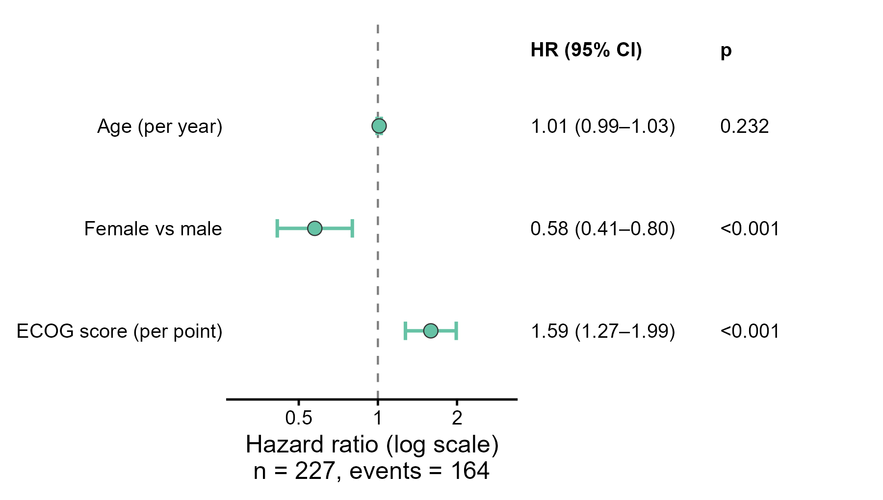
Cox 回归森林图(风险比 HR 与 95% 置信区间,对数轴)
GAL-0010
把 Cox 比例风险回归中各变量的风险比(HR)及其 95% 置信区间画在对数坐标轴上,以 HR = 1 为参考线,一眼看出各因素与生存风险的关联方向和精度。
图与代码
code/R/main.R
suppressPackageStartupMessages({
  library(ggplot2)
  library(survival)
})

d <- na.omit(read.csv("data/lung.csv", encoding = "UTF-8"))   # 去掉 ph.ecog 缺失的观测
d$event <- as.integer(d$status == 2)                          # lung:status 1 = 删失,2 = 死亡
d$female <- as.integer(d$sex == 2)                            # 女性 vs 男性

fit <- coxph(Surv(time, event) ~ age + female + ph.ecog, data = d, ties = "efron")
cf <- summary(fit)$coefficients
z <- qnorm(0.975)
res <- data.frame(
  term = rownames(cf), coef = cf[, "coef"], se = cf[, "se(coef)"], p = cf[, "Pr(>|z|)"],
  hr = exp(cf[, "coef"]), lo = exp(cf[, "coef"] - z * cf[, "se(coef)"]), hi = exp(cf[, "coef"] + z * cf[, "se(coef)"]),
  row.names = NULL)
res$label <- c("Age (per year)", "Female vs male", "ECOG score (per point)")
res$y <- 3:1
res$hr_txt <- sprintf("%.2f (%.2f–%.2f)", res$hr, res$lo, res$hi)
res$p_txt <- ifelse(res$p < 0.001, "<0.001", ifelse(res$p < 0.01, sprintf("%.4f", signif(res$p, 2)), sprintf("%.3f", res$p)))
write.csv(rbind(res[, c("term", "coef", "se", "p", "hr", "lo", "hi")],
                data.frame(term = c("n", "events"), coef = c(nrow(d), sum(d$event)), se = NA, p = NA, hr = NA, lo = NA, hi = NA)),
          "outputs/stats_r.csv", row.names = FALSE)

p <- ggplot(res, aes(x = hr, y = y)) +
  geom_vline(xintercept = 1, linetype = "dashed", colour = "grey50", linewidth = 0.5) +
  geom_errorbar(aes(xmin = lo, xmax = hi), orientation = "y", width = 0.18, colour = "#66C2A5", linewidth = 0.8) +
  geom_point(size = 3, shape = 21, fill = "#66C2A5", colour = "grey20", stroke = 0.4) +
  geom_text(aes(x = 3.8, label = hr_txt), hjust = 0, size = 3.4) +
  geom_text(aes(x = 20, label = p_txt), hjust = 0, size = 3.4) +
  annotate("text", x = 3.8, y = 3.75, label = "HR (95% CI)", hjust = 0, size = 3.4, fontface = "bold") +
  annotate("text", x = 20, y = 3.75, label = "p", hjust = 0, size = 3.4, fontface = "bold") +
  scale_x_log10(breaks = c(0.5, 1, 2), labels = c("0.5", "1", "2")) +
  scale_y_continuous(breaks = res$y, labels = res$label) +
  coord_cartesian(xlim = c(0.3, 3), ylim = c(0.5, 3.9), clip = "off") +
  labs(x = sprintf("Hazard ratio (log scale)\nn = %d, events = %d", nrow(d), sum(d$event)), y = NULL) +
  theme_classic(base_size = 12) +
  theme(axis.text.y = element_text(colour = "black"), axis.line.y = element_blank(), axis.ticks.y = element_blank(),
        plot.margin = margin(8, 180, 8, 8))

ggsave("outputs/figure_r.png", p, width = 6, height = 3.4, dpi = 300, bg = "white")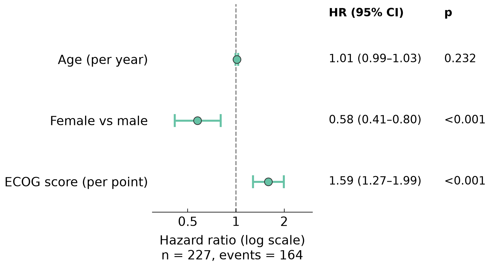
code/py/main.py
import numpy as np
import pandas as pd
import matplotlib.pyplot as plt
import scienceplots  # noqa: F401
from lifelines import CoxPHFitter

plt.style.use(["science", "no-latex"])
plt.rcParams["font.family"] = "sans-serif"

d = pd.read_csv("data/lung.csv").dropna().copy()   # 去掉 ph.ecog 缺失的观测
d["event"] = (d["status"] == 2).astype(int)        # lung:status 1 = 删失,2 = 死亡
d["female"] = (d["sex"] == 2).astype(int)          # 女性 vs 男性
d = d.rename(columns={"ph.ecog": "ph_ecog"})

cph = CoxPHFitter().fit(d[["time", "event", "age", "female", "ph_ecog"]], duration_col="time", event_col="event")
s = cph.summary.loc[["age", "female", "ph_ecog"]]
z = 1.959963984540054
res = pd.DataFrame({"term": ["age", "female", "ph.ecog"], "coef": s["coef"].to_numpy(), "se": s["se(coef)"].to_numpy(),
                    "p": s["p"].to_numpy()})
res["hr"] = np.exp(res["coef"])
res["lo"] = np.exp(res["coef"] - z * res["se"])
res["hi"] = np.exp(res["coef"] + z * res["se"])
pd.concat([res, pd.DataFrame({"term": ["n", "events"], "coef": [len(d), d["event"].sum()]})]).to_csv(
    "outputs/stats_py.csv", index=False)

labels = ["Age (per year)", "Female vs male", "ECOG score (per point)"]
ys = [3, 2, 1]
fig, ax = plt.subplots(figsize=(6, 3.4))
ax.axvline(1, linestyle="--", color="#7F7F7F", lw=0.9, zorder=0)
for y, r in zip(ys, res.itertuples()):
    ax.plot([r.lo, r.hi], [y, y], color="#66C2A5", lw=1.6, solid_capstyle="butt")
    ax.plot([r.lo, r.lo], [y - 0.09, y + 0.09], color="#66C2A5", lw=1.6)
    ax.plot([r.hi, r.hi], [y - 0.09, y + 0.09], color="#66C2A5", lw=1.6)
    ax.scatter([r.hr], [y], s=40, facecolor="#66C2A5", edgecolor="#333333", linewidth=0.6, zorder=3)
    p_txt = "<0.001" if r.p < 0.001 else (f"{float(f'{r.p:.2g}'):.4f}" if r.p < 0.01 else f"{r.p:.3f}")
    ax.text(3.8, y, f"{r.hr:.2f} ({r.lo:.2f}–{r.hi:.2f})", ha="left", va="center", fontsize=9, clip_on=False)
    ax.text(20, y, p_txt, ha="left", va="center", fontsize=9, clip_on=False)
ax.text(3.8, 3.75, "HR (95% CI)", ha="left", va="center", fontsize=9, fontweight="bold", clip_on=False)
ax.text(20, 3.75, "p", ha="left", va="center", fontsize=9, fontweight="bold", clip_on=False)

ax.set_xscale("log")
ax.set_xlim(0.3, 3)
ax.set_ylim(0.5, 3.9)
ax.set_xticks([0.5, 1, 2], ["0.5", "1", "2"])
ax.set_yticks(ys, labels)
ax.minorticks_off()
ax.tick_params(axis="y", left=False, right=False)
ax.tick_params(axis="x", top=False)
for sp in ("top", "right", "left"):
    ax.spines[sp].set_visible(False)
ax.set_xlabel(f"Hazard ratio (log scale)\nn = {len(d)}, events = {int(d['event'].sum())}")
fig.subplots_adjust(left=0.30, right=0.60, bottom=0.27, top=0.96)
fig.savefig("outputs/figure_py.png", dpi=300, facecolor="white")
什么时候用
- 汇报多因素 Cox 回归结果,让读者快速比较各变量的效应方向与不确定性
- 在论文或汇报中替代冗长的回归系数表
- 区间是否跨过 1 可直观提示该变量在统计上是否显著(需结合 p 值与临床意义)
常见误用
- HR 必须画在对数轴上,使 0.5 与 2 关于 1 对称;用线性轴会让保护与有害效应在视觉上失衡
- 连续变量的 HR 对应“每增加一个单位”(本例年龄为每岁、ECOG 评分为每 1 分),单位不同的 HR 大小不能直接比较
- 本例的 ECOG 评分按连续变量处理,隐含“每增加 1 分风险按相同倍数增加”的线性假设(纳入的 227 例中 ECOG 0、1、2、3 分分别为 63、113、50、1 例,3 分只有 1 例,不宜再拆成分类变量);各 HR 均为多因素调整后的结果,且未检验比例风险假设(如 cox.zph)
- HR 是相对指标,不给出绝对风险;区间跨过 1 不等于“没有关联”,只是本样本下证据不足;数据来自观察性研究,不能据此作因果解释
数据与下载
数据:R 包 survival 内置数据集 lung(晚期肺癌患者生存数据)(R 包 survival 随 CRAN 分发(LGPL-2 | LGPL-3))。结局为总生存(time 为天数;status:1 = 删失,2 = 死亡);协变量为年龄 age、性别(sex:1 = 男,2 = 女,代码中取女 vs 男)与 ECOG 体能评分 ph.ecog(0~3,按连续变量)。 去除 ph.ecog 缺失的 1 例后纳入 227 例。HR 与 Wald 95% 置信区间由代码根据 Cox 模型(Efron 法处理结点)的系数和标准误计算。
下载包 sha256:46769e515e0a12732ea2ce81b224bd68d3b255f346318b90621a91be5fb76bfe