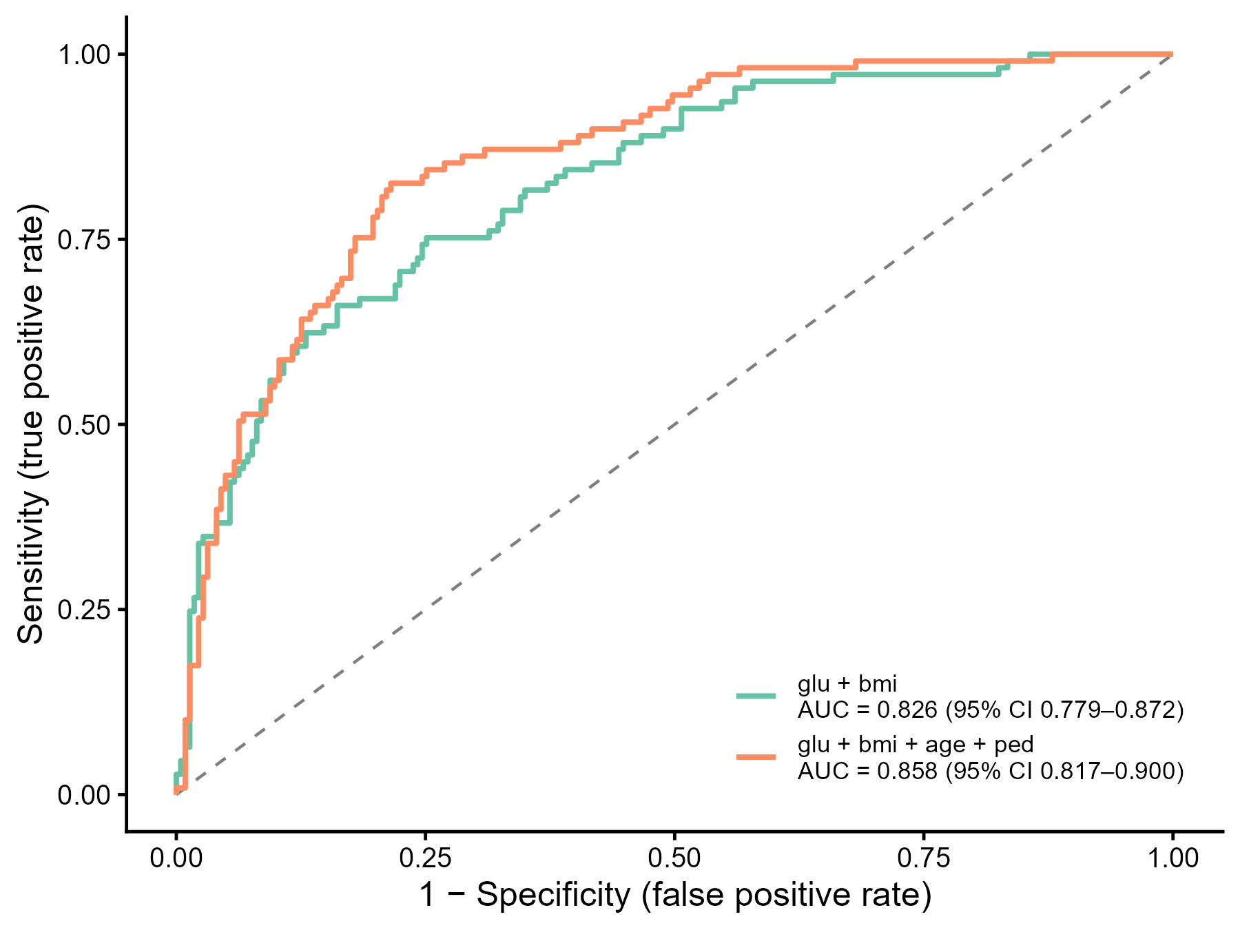
ROC 曲线(两个模型的比较,含 AUC 与 95% 置信区间)
GAL-0008
在独立的测试集上,用 ROC 曲线比较两个逻辑回归模型的区分能力(discrimination),并标注 AUC 及其 DeLong 95% 置信区间。
图与代码
code/R/main.R
suppressPackageStartupMessages({
  library(ggplot2)
  library(pROC)
})

tr <- read.csv("data/pima_tr.csv", encoding = "UTF-8")
te <- read.csv("data/pima_te.csv", encoding = "UTF-8")
tr$y <- as.integer(tr$type == "Yes")
te$y <- as.integer(te$type == "Yes")

# 训练集上拟合两个逻辑回归,在独立的测试集上评价
f <- list(`glu + bmi` = y ~ glu + bmi, `glu + bmi + age + ped` = y ~ glu + bmi + age + ped)
cols <- c("#66C2A5", "#FC8D62")
curves <- list(); labs_ <- c(); stats <- list()
for (i in seq_along(f)) {
  m <- glm(f[[i]], family = binomial, data = tr)
  pred <- predict(m, newdata = te, type = "response")
  r <- roc(te$y, pred, levels = c(0, 1), direction = "<", quiet = TRUE)
  ci <- as.numeric(ci.auc(r, method = "delong"))   # DeLong 95% 置信区间:下限、AUC、上限
  nm <- names(f)[i]
  labs_[nm] <- sprintf("%s\nAUC = %.3f (95%% CI %.3f–%.3f)", nm, ci[2], ci[1], ci[3])
  curves[[nm]] <- data.frame(fpr = 1 - r$specificities, tpr = r$sensitivities, model = nm)
  stats[[i]] <- data.frame(key = c(paste0("m", i, "_coef_", names(coef(m))), paste0("m", i, c("_auc", "_ci_lo", "_ci_hi"))),
                           value = c(unname(coef(m)), ci[2], ci[1], ci[3]))
}
write.csv(do.call(rbind, stats), "outputs/stats_r.csv", row.names = FALSE)
curves <- do.call(rbind, curves)
curves$model <- factor(curves$model, levels = names(f), labels = labs_)

p <- ggplot(curves, aes(fpr, tpr, colour = model)) +
  annotate("segment", x = 0, y = 0, xend = 1, yend = 1, linetype = "dashed", colour = "grey50", linewidth = 0.5) +
  geom_path(linewidth = 0.9) +
  scale_colour_manual(values = cols, name = NULL) +
  scale_x_continuous(limits = c(0, 1), breaks = seq(0, 1, 0.25)) +
  scale_y_continuous(limits = c(0, 1), breaks = seq(0, 1, 0.25)) +
  labs(x = "1 − Specificity (false positive rate)", y = "Sensitivity (true positive rate)") +
  theme_classic(base_size = 12) +
  theme(legend.position = "inside", legend.position.inside = c(0.98, 0.04), legend.justification = c(1, 0),
        legend.text = element_text(size = 8.5), legend.key.spacing.y = unit(4, "pt"))

ggsave("outputs/figure_r.png", p, width = 6, height = 4.5, dpi = 300, bg = "white")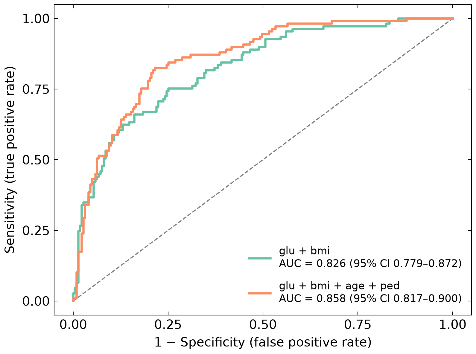
code/py/main.py
import numpy as np
import pandas as pd
import matplotlib.pyplot as plt
import scienceplots  # noqa: F401
import statsmodels.api as sm
from sklearn.metrics import roc_curve, roc_auc_score

plt.style.use(["science", "no-latex"])
plt.rcParams["font.family"] = "sans-serif"

tr = pd.read_csv("data/pima_tr.csv")
te = pd.read_csv("data/pima_te.csv")
tr["y"] = (tr["type"] == "Yes").astype(int)
te["y"] = (te["type"] == "Yes").astype(int)


def delong_auc_ci(y, s, z=1.959963984540054):
    """DeLong 法的 AUC 方差与 95% 置信区间(自写,按 DeLong 等 1988 的结构分量公式;样本小,直接用成对比较矩阵)。"""
    pos, neg = s[y == 1], s[y == 0]
    psi = (pos[:, None] > neg[None, :]) + 0.5 * (pos[:, None] == neg[None, :])
    auc = psi.mean()
    var = psi.mean(axis=1).var(ddof=1) / len(pos) + psi.mean(axis=0).var(ddof=1) / len(neg)
    se = np.sqrt(var)
    return auc, max(auc - z * se, 0.0), min(auc + z * se, 1.0)


# 训练集上拟合两个逻辑回归,在独立的测试集上评价
f = {"glu + bmi": ["glu", "bmi"], "glu + bmi + age + ped": ["glu", "bmi", "age", "ped"]}
cols = ["#66C2A5", "#FC8D62"]
fig, ax = plt.subplots(figsize=(6, 4.5))
ax.plot([0, 1], [0, 1], linestyle="--", color="#7F7F7F", lw=0.9)
rows = []
for i, (nm, xs) in enumerate(f.items(), start=1):
    m = sm.Logit(tr["y"], sm.add_constant(tr[xs])).fit(disp=0)
    pred = m.predict(sm.add_constant(te[xs])).to_numpy()
    fpr, tpr, _ = roc_curve(te["y"], pred, drop_intermediate=False)
    auc_sk = roc_auc_score(te["y"], pred)
    auc, lo, hi = delong_auc_ci(te["y"].to_numpy(), pred)
    assert abs(auc - auc_sk) < 1e-12
    rows += [(f"m{i}_coef_{'(Intercept)' if k == 'const' else k}", v) for k, v in m.params.items()]
    rows += [(f"m{i}_auc", auc_sk), (f"m{i}_ci_lo", lo), (f"m{i}_ci_hi", hi)]
    ax.plot(fpr, tpr, color=cols[i - 1], lw=1.8,
            label=f"{nm}\nAUC = {auc_sk:.3f} (95% CI {lo:.3f}–{hi:.3f})")
pd.DataFrame(rows, columns=["key", "value"]).to_csv("outputs/stats_py.csv", index=False)

ax.set_xlim(-0.05, 1.05)
ax.set_ylim(-0.05, 1.05)
ax.set_xticks(np.arange(0, 1.01, 0.25))
ax.set_yticks(np.arange(0, 1.01, 0.25))
ax.set_xlabel("1 − Specificity (false positive rate)")
ax.set_ylabel("Sensitivity (true positive rate)")
ax.legend(loc="lower right", frameon=False, fontsize=8.5, labelspacing=0.9)
ax.minorticks_off()
fig.savefig("outputs/figure_py.png", dpi=300, facecolor="white")
什么时候用
- 评价诊断或预测模型区分“有病/无病”(二分类结局)的能力
- 比较两个及以上模型(如增加预测变量前后)的区分度
- 展示模型在所有可能阈值下灵敏度与特异度的权衡
常见误用
- AUC 只衡量区分度,不反映预测概率是否准确;需另做校准评价(见 GAL-0009),ROC 曲线也不直接给出临床上应取的阈值
- 应在独立数据上评价(本例用 Pima.tr 拟合、Pima.te 评价);在拟合数据上直接算 AUC 会高估
- 两个模型的 AUC 置信区间有重叠,不等于“无差异”或“有差异”;比较两个相关 ROC 曲线应使用配对检验(如 DeLong 检验),本图未做该检验,不能据此宣称某模型更优
- 当结局极不平衡时,ROC 曲线可能显得过于乐观,可结合精确率–召回率曲线与决策曲线分析
数据与下载
数据:R 包 MASS 内置数据集 Pima.tr(训练,200 例)与 Pima.te(测试,332 例)(皮马印第安女性糖尿病数据)(R 包 MASS 随 CRAN 分发(GPL-2 | GPL-3))。结局 type(Yes = 糖尿病);预测变量为血浆葡萄糖 glu、体重指数 bmi、年龄 age、糖尿病家系函数 ped。 在 Pima.tr 上用 glm 逻辑回归拟合两个模型(模型 1:glu + bmi;模型 2:glu + bmi + age + ped),在 Pima.te 上计算 ROC。 R 版用 pROC 计算 ROC 与 DeLong 置信区间;Python 版用 statsmodels 拟合、scikit-learn 计算曲线与 AUC,DeLong 置信区间为自写实现(两版数值一致)。
下载包 sha256:5a43dee928fea6bf34404fe582c71a91b9aa249955301b911fdaf10edab33e8b