GSEA 加权富集运行曲线(ES 教学示例)
GAL-0025
用透明模拟的有序基因列表展示 GSEA 加权运行分数:上方曲线是 ES 的累积过程,中间标出基因集命中位置,下方显示排序指标。本例只独立计算和绘制原始 ES,不计算 NES、P 值或 FDR,也不声称完成了完整的 GSEA 显著性分析。
图与代码
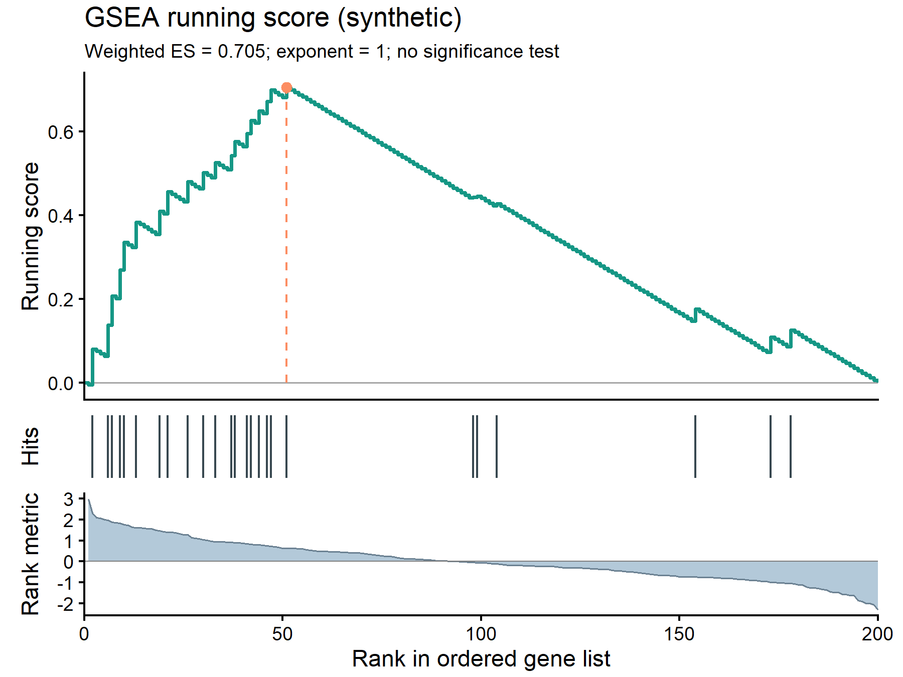
code/R/main.R
suppressPackageStartupMessages(library(ggplot2))

running_es <- function(score, hit) {
  stopifnot(length(score) == length(hit), all(is.finite(score)), all(hit %in% c(0, 1)))
  nh <- sum(hit)
  stopifnot(nh > 0, nh < length(hit), sum(abs(score[hit == 1])) > 0)
  step <- ifelse(hit == 1, abs(score) / sum(abs(score[hit == 1])), -1 / (length(hit) - nh))
  cumsum(step)
}
stopifnot(isTRUE(all.equal(running_es(c(4, 3, 2, 1), c(1, 0, 1, 0)), c(2/3, 1/6, 1/2, 0))))

dir.create("outputs", showWarnings = FALSE)
d <- read.csv("data/ranked_genes.csv")
genes <- read.csv("data/gene_set.csv")$gene
stopifnot(!anyDuplicated(d$gene), !anyDuplicated(genes), all(genes %in% d$gene))
d <- d[order(-d$score, d$gene), ]
d$rank <- seq_len(nrow(d))
d$hit <- as.integer(d$gene %in% genes)
d$running <- running_es(d$score, d$hit)
peak <- which.max(abs(d$running))
es <- d$running[peak]
stats <- data.frame(key = c("n", "n_hit", "weight_exponent", "es", "peak_rank", "terminal_score"),
                    value = c(nrow(d), sum(d$hit), 1, es, peak, tail(d$running, 1)))
write.csv(stats, "outputs/stats_r.csv", row.names = FALSE)
write.csv(d[, c("rank", "hit", "running")], "outputs/curve_r.csv", row.names = FALSE)
numbers <- lapply(seq_len(nrow(stats)), function(i) list(id = stats$key[i], value = stats$value[i],
  display = if (stats$key[i] == "terminal_score") sprintf("%.0f", round(stats$value[i], 12) + 0) else sprintf(if (stats$key[i] == "es") "%.3f" else "%.0f", stats$value[i]),
  source = list(type = "computed", locator = "code/R/main.R")))
jsonlite::write_json(list(schema = "zzy-media-studio/numbers/v1", asset = "GAL-0025", numbers = numbers),
  "outputs/numbers.json", auto_unbox = TRUE, pretty = TRUE, digits = 16)
curve <- rbind(data.frame(rank = 0, running = 0), d[, c("rank", "running")])
base <- theme_classic(base_size = 11) + theme(plot.margin = margin(3, 12, 3, 10))
p1 <- ggplot(curve, aes(rank, running)) +
  geom_hline(yintercept = 0, colour = "grey65", linewidth = 0.4) +
  geom_step(colour = "#159785", linewidth = 0.85) +
  annotate("segment", x = peak, xend = peak, y = 0, yend = es, linetype = "dashed", colour = "#FC8D62") +
  geom_point(data = data.frame(rank = peak, running = es), size = 2, colour = "#FC8D62") +
  scale_x_continuous(limits = c(0, nrow(d)), expand = c(0, 0)) +
  labs(title = "GSEA running score (synthetic)",
       subtitle = sprintf("Weighted ES = %.3f; exponent = 1; no significance test", es),
       y = "Running score", x = NULL) + base +
  theme(axis.text.x = element_blank(), axis.ticks.x = element_blank(),
        plot.title = element_text(size = 13), plot.subtitle = element_text(size = 9))
p2 <- ggplot(d[d$hit == 1, ], aes(rank)) +
  geom_segment(aes(xend = rank, y = 0, yend = 1), linewidth = 0.45, colour = "#37474F") +
  scale_x_continuous(limits = c(0, nrow(d)), expand = c(0, 0)) +
  scale_y_continuous(breaks = NULL) + labs(x = NULL, y = "Hits") + base +
  theme(axis.text.x = element_blank(), axis.ticks = element_blank(), axis.line = element_blank())
p3 <- ggplot(d, aes(rank, score)) +
  geom_area(fill = "#B3C9D9", colour = "#6B8192", linewidth = 0.35) +
  geom_hline(yintercept = 0, colour = "grey50", linewidth = 0.3) +
  scale_x_continuous(limits = c(0, nrow(d)), expand = c(0, 0)) +
  labs(x = "Rank in ordered gene list", y = "Rank metric") + base
png("outputs/figure_r.png", width = 6, height = 4.5, units = "in", res = 300, bg = "white")
plots <- lapply(list(p1, p2, p3), ggplotGrob)
widths <- do.call(grid::unit.pmax, lapply(plots, function(p) p$widths))
plots <- lapply(plots, function(p) { p$widths <- widths; p })
grid::grid.newpage()
grid::pushViewport(grid::viewport(layout = grid::grid.layout(3, 1, heights = grid::unit(c(0.60, 0.12, 0.28), "null"))))
for (i in 1:3) grid::grid.draw(grid::editGrob(plots[[i]], vp = grid::viewport(layout.pos.row = i)))
dev.off()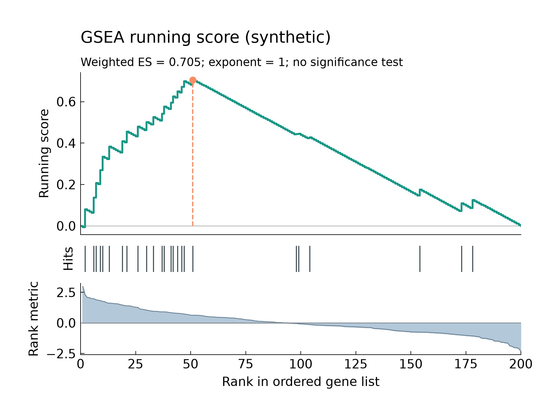
code/py/main.py
from pathlib import Path

import numpy as np
import pandas as pd
import matplotlib.pyplot as plt
import scienceplots  # noqa: F401


def running_es(score, hit):
    score, hit = np.asarray(score, float), np.asarray(hit)
    if score.ndim != 1 or score.shape != hit.shape or not np.isfinite(score).all() or not np.isin(hit, [0, 1]).all():
        raise ValueError("指标与命中必须为等长有限数值向量,命中只能为0/1")
    nh = int(hit.sum())
    weight = np.abs(score[hit == 1]).sum()
    if not 0 < nh < len(hit) or weight <= 0:
        raise ValueError("命中数必须介于0与N之间,命中权重总和必须大于0")
    return np.cumsum(np.where(hit == 1, np.abs(score) / weight, -1 / (len(hit) - nh)))


def main():
    Path("outputs").mkdir(exist_ok=True)
    d = pd.read_csv("data/ranked_genes.csv")
    genes = pd.read_csv("data/gene_set.csv").gene
    if d.gene.duplicated().any() or genes.duplicated().any() or not genes.isin(d.gene).all():
        raise ValueError("基因ID必须唯一且集合必须位于排序列表中")
    d = d.sort_values(["score", "gene"], ascending=[False, True]).reset_index(drop=True)
    d["rank"] = np.arange(1, len(d) + 1)
    d["hit"] = d.gene.isin(genes).astype(int)
    d["running"] = running_es(d.score, d.hit)
    peak = int(np.argmax(np.abs(d.running)))
    es = float(d.running.iloc[peak])
    pd.DataFrame({"key": ["n", "n_hit", "weight_exponent", "es", "peak_rank", "terminal_score"],
                  "value": [len(d), d.hit.sum(), 1, es, peak + 1, d.running.iloc[-1]]}).to_csv("outputs/stats_py.csv", index=False)
    d[["rank", "hit", "running"]].to_csv("outputs/curve_py.csv", index=False)

    plt.style.use(["science", "no-latex"])
    plt.rcParams.update({"font.family": "sans-serif", "savefig.bbox": "standard", "font.size": 10})
    fig, axes = plt.subplots(3, 1, figsize=(6, 4.5), sharex=True, gridspec_kw={"height_ratios": [3.4, 0.55, 1.5]})
    ax, rug, metric = axes
    ax.axhline(0, color="0.65", lw=0.5)
    ax.step(np.r_[0, d["rank"]], np.r_[0, d.running], where="post", color="#159785", lw=1.5)
    ax.vlines(peak + 1, 0, es, colors="#FC8D62", linestyles="--", lw=1)
    ax.scatter([peak + 1], [es], s=22, c="#FC8D62", zorder=4)
    ax.set_ylabel("Running score")
    ax.set_title("GSEA running score (synthetic)", loc="left", fontsize=13, pad=24)
    ax.text(0, 1.04, f"Weighted ES = {es:.3f}; exponent = 1; no significance test", transform=ax.transAxes, fontsize=9)
    rug.vlines(d.loc[d.hit == 1, "rank"], 0, 1, color="#37474F", lw=0.8)
    rug.set(ylim=(0, 1), yticks=[], ylabel="Hits")
    for spine in rug.spines.values():
        spine.set_visible(False)
    metric.fill_between(d["rank"], d.score, color="#B3C9D9")
    metric.plot(d["rank"], d.score, color="#6B8192", lw=0.6)
    metric.axhline(0, color="0.5", lw=0.5)
    metric.set(xlabel="Rank in ordered gene list", ylabel="Rank metric", xlim=(0, len(d)))
    for a in axes:
        a.spines[["top", "right"]].set_visible(False)
        a.minorticks_off()
        a.tick_params(top=False, right=False)
    ax.tick_params(axis="x", which="both", bottom=False, labelbottom=False)
    rug.tick_params(axis="x", which="both", bottom=False, labelbottom=False)
    fig.subplots_adjust(left=0.15, right=0.97, bottom=0.12, top=0.82, hspace=0.13)
    fig.savefig("outputs/figure_py.png", dpi=300, facecolor="white")
    plt.close(fig)


if __name__ == "__main__":
    main()
什么时候用
- 学习有序基因列表中“命中加分、未命中扣分”的加权 ES 定义
- 在绘制正式富集结果前核对基因 ID、排序方向、命中位置和权重含义
- 为 R 和 Python 的同一运行分数实现提供可复核的小例子
常见误用
- 本例基因名、排序指标和基因集均为模拟,不对应真实生物过程,也不能用于报告通路激活
- ES 不是 NES,更不是显著性;正式分析还需预先指定置换类型、置换次数、归一化及多重比较方法,本例不计算这些结果
- 排序指标由大到小排列;命中权重为指标绝对值的一次方,并除以命中权重总和,未命中每次扣除 1/(N−Nh)
- 输入必须为唯一基因 ID,基因集全部位于排序列表中,且命中数介于 0 与列表长度之间;并列分数按基因 ID 排序仅为保证确定性,正式分析须检查并列排名的敏感性
数据与下载
数据:本项目原创模拟数据,由 code/R/make_data.R 固定种子 20261026 生成(CC0-1.0(本项目原创模拟教学数据))。ranked_genes.csv 是 200 个模拟基因的连续排序指标;gene_set.csv 是 25 个模拟基因组成的教学集合。不是 GO、KEGG 或 MSigDB 数据,也没有复用真实受试者或原论文数据。
下载包 sha256:6a8ff3f6f935b872d730c39f1827663876556675299c3ffc6180837d7b6a2bd1