决策曲线DCA(阈值与净获益)
GAL-0023
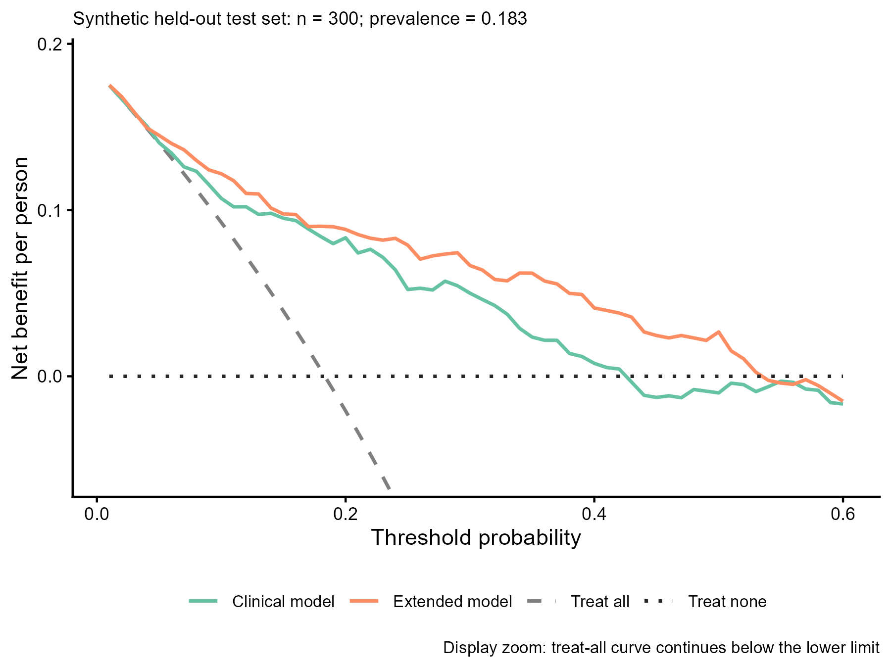
在独立模拟测试集上,用阈值概率体现假阳性代价,比较两个模型与全部处理、全部不处理策略的净获益。展示二分类结局的决策曲线,不推断实际临床可用性。
图与代码
code/R/main.R
suppressPackageStartupMessages(library(ggplot2))
dir.create("outputs", showWarnings = FALSE)
net_benefit <- function(y, probability, threshold) {
  stopifnot(length(y) == length(probability), length(y) > 0, all(y %in% c(0, 1)),
            all(is.finite(probability)), all(probability >= 0 & probability <= 1),
            all(is.finite(threshold)), all(threshold > 0 & threshold < 1))
  vapply(threshold, function(t) {
    selected <- probability >= t
    (sum(y[selected] == 1) - sum(y[selected] == 0) * t / (1 - t)) / length(y)
  }, numeric(1))
}
stopifnot(abs(net_benefit(c(1, 0, 1, 0), c(.9, .7, .4, .1), .5) - 0) < 1e-12)
stopifnot(abs(net_benefit(c(1, 0, 1, 0), c(.9, .7, .4, .1), .25) - 5/12) < 1e-12)
stopifnot(abs(net_benefit(c(1, 0), c(.29, .1), .29) - .5) < 1e-12)
d <- read.csv("data/test_predictions.csv")
# 用整数格点除以100,避免 seq 的浮点累积改变恰好等于阈值的分类。
t <- (1:60) / 100
curves <- rbind(data.frame(threshold = t, model = "clinical", net_benefit = net_benefit(d$y, d$clinical, t)),
                data.frame(threshold = t, model = "extended", net_benefit = net_benefit(d$y, d$extended, t)),
                data.frame(threshold = t, model = "all", net_benefit = mean(d$y) - (1 - mean(d$y)) * t/(1 - t)),
                data.frame(threshold = t, model = "none", net_benefit = 0))
write.csv(curves, "outputs/curves_r.csv", row.names = FALSE)
write.csv(data.frame(key = c("n_test", "n_positive", "prevalence"), value = c(nrow(d), sum(d$y), mean(d$y))),
          "outputs/stats_r.csv", row.names = FALSE)
p <- ggplot(curves, aes(threshold, net_benefit, colour = model, linetype = model)) +
  geom_line(linewidth = .8) +
  scale_colour_manual(values = c(clinical = "#66C2A5", extended = "#FC8D62", all = "grey50", none = "grey15"),
                      breaks = c("clinical", "extended", "all", "none"),
                      labels = c("Clinical model", "Extended model", "Treat all", "Treat none"), name = NULL) +
  scale_linetype_manual(values = c(clinical = "solid", extended = "solid", all = "dashed", none = "dotted"),
                        breaks = c("clinical", "extended", "all", "none"),
                        labels = c("Clinical model", "Extended model", "Treat all", "Treat none"), name = NULL) +
  coord_cartesian(ylim = c(-.06, max(curves$net_benefit) + .015)) +
  labs(x = "Threshold probability", y = "Net benefit per person",
       subtitle = sprintf("Synthetic held-out test set: n = %d; prevalence = %.3f", nrow(d), mean(d$y)),
       caption = "Display zoom: treat-all curve continues below the lower limit") +
  theme_classic(base_size = 11) + theme(legend.position = "bottom", legend.text = element_text(size = 8),
                                      plot.subtitle = element_text(size = 9), plot.caption = element_text(size = 8))
ggsave("outputs/figure_r.png", p, width = 6, height = 4.5, dpi = 300, bg = "white")

# 账本从本次计算的统计表生成,显示精度与图中标注一致。
ledger_stats <- read.csv("outputs/stats_r.csv")
ledger_numbers <- lapply(seq_len(nrow(ledger_stats)), function(i) {
  key <- ledger_stats$key[i]
  value <- ledger_stats$value[i]
  list(id = key, value = value,
       display = if (startsWith(key, "n_")) sprintf("%.0f", value) else sprintf("%.3f", value),
       source = list(type = "computed", locator = "code/R/main.R -> outputs/stats_r.csv"))
})
jsonlite::write_json(list(schema = "zzy-media-studio/numbers/v1", asset = "GAL-0023", numbers = ledger_numbers),
                     "outputs/numbers.json", auto_unbox = TRUE, pretty = TRUE, digits = 16)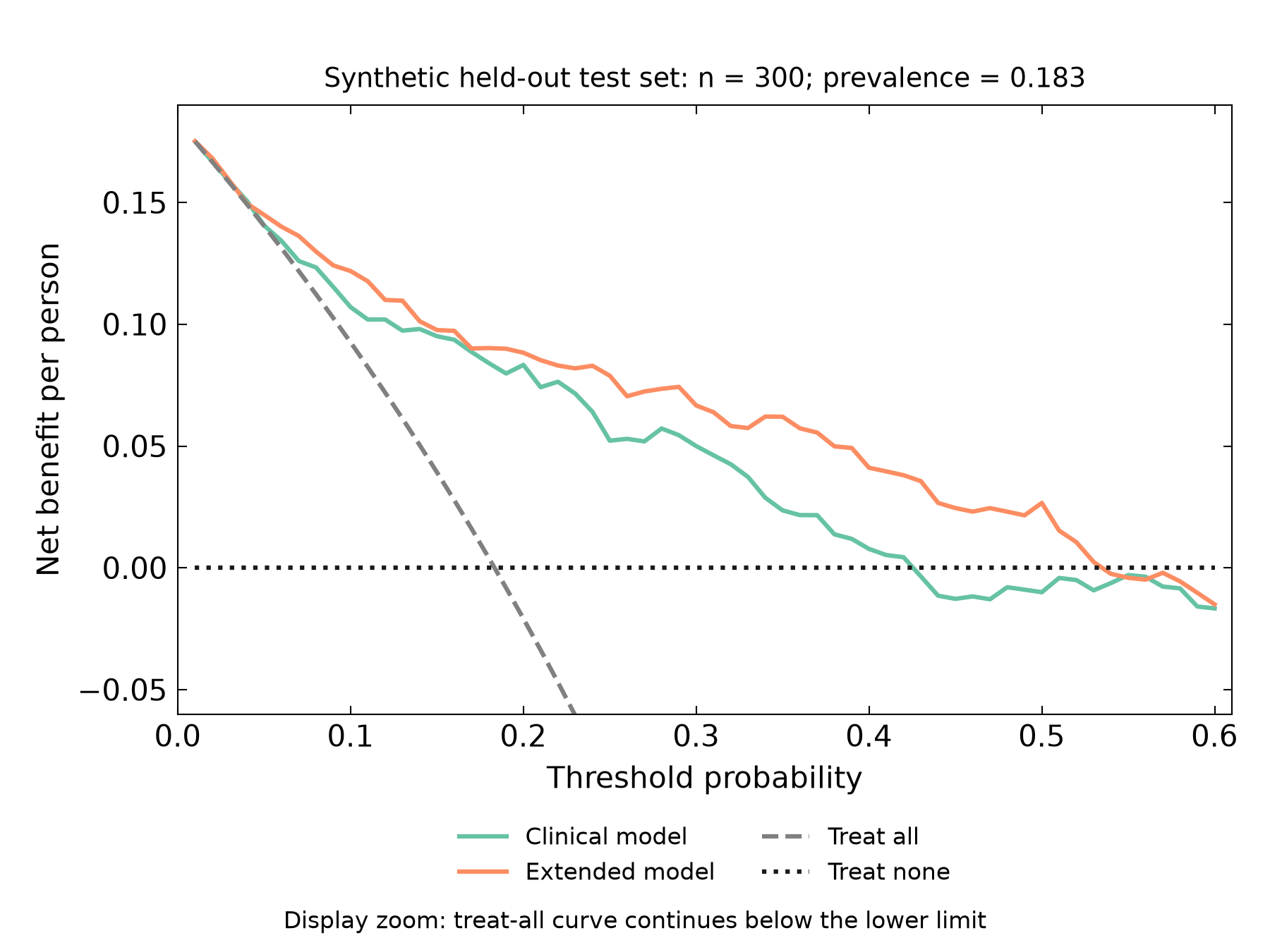
code/py/main.py
from pathlib import Path
import numpy as np
import pandas as pd
import matplotlib.pyplot as plt
import scienceplots

plt.style.use(["science", "no-latex"])
plt.rcParams["font.family"] = "sans-serif"
plt.rcParams["savefig.bbox"] = "standard"

def net_benefit(y, probability, threshold):
    y, probability, threshold = np.asarray(y), np.asarray(probability), np.atleast_1d(threshold)
    if len(y) == 0 or len(y) != len(probability) or not np.isin(y, [0, 1]).all() or not np.isfinite(probability).all() or not ((probability >= 0) & (probability <= 1)).all() or not np.isfinite(threshold).all() or not ((threshold > 0) & (threshold < 1)).all():
        raise ValueError("Need binary outcomes, probabilities in [0,1], and thresholds in (0,1)")
    selected = probability[:, None] >= threshold[None, :]
    tp = ((y[:, None] == 1) & selected).sum(axis=0)
    fp = ((y[:, None] == 0) & selected).sum(axis=0)
    return (tp - fp * threshold / (1 - threshold)) / len(y)


def main():
    Path("outputs").mkdir(exist_ok=True)
    d = pd.read_csv("data/test_predictions.csv")
    t = np.arange(1, 61) / 100
    fig, ax = plt.subplots(figsize=(6, 4.5))
    fig.subplots_adjust(left=.14, right=.97, bottom=.25, top=.89)
    curves = []
    for nm, label, col, ls in [("clinical", "Clinical model", "#66C2A5", "-"), ("extended", "Extended model", "#FC8D62", "-"), ("all", "Treat all", ".5", "--"), ("none", "Treat none", ".1", ":")]:
        nb = d.y.mean() - (1-d.y.mean())*t/(1-t) if nm == "all" else np.zeros(len(t)) if nm == "none" else net_benefit(d.y, d[nm], t)
        curves.append(pd.DataFrame({"threshold": t, "model": nm, "net_benefit": nb}))
        ax.plot(t, nb, color=col, ls=ls, lw=1.5, label=label)
    ax.set(xlim=(0, .61), ylim=(-.06, max(c.net_benefit.max() for c in curves)+.015), xlabel="Threshold probability", ylabel="Net benefit per person")
    ax.minorticks_off()
    ax.set_title(f"Synthetic held-out test set: n = {len(d)}; prevalence = {d.y.mean():.3f}", fontsize=9)
    ax.legend(loc="upper center", bbox_to_anchor=(.5, -.15), ncol=2, frameon=False, fontsize=8)
    fig.text(.5, .025, "Display zoom: treat-all curve continues below the lower limit", ha="center", fontsize=8)
    pd.concat(curves, ignore_index=True).to_csv("outputs/curves_py.csv", index=False)
    pd.DataFrame([("n_test", len(d)), ("n_positive", d.y.sum()), ("prevalence", d.y.mean())], columns=["key", "value"]).to_csv("outputs/stats_py.csv", index=False)
    fig.savefig("outputs/figure_py.png", dpi=300, facecolor="white")
    plt.close(fig)


if __name__ == "__main__":
    main()
什么时候用
- 模型已输出概率,需要在有意义的决策阈值范围比较策略
- 希望补充区分度指标,解释假阳性代价与潜在收益
常见误用
- 净获益=TP/n−FP/n×t/(1−t),阈值 t 严格处于 0 与 1 之间;使用预测概率,不是预先二值化标签
- 全部处理和全部不处理是参照策略;本例仅二分类结局,不能照搬到删失生存数据
- 阈值范围是教学展示,不是临床推荐;模型训练/评价分离,未做净获益置信区间
- 纵轴放大以便比较模型,全部处理曲线在高阈值时低于图框;完整值见 curves CSV
- 模拟教学数据不代表真实患者,净获益为每人尺度,不是准确率或真实避免治疗人数
数据与下载
数据:固定种子 20261026 的 R 原创模拟,与 GAL-0022 相同生成机制、各包完整自包含(原创模拟数据,CC0-1.0(教学用途,非真实患者))。make_data.R 生成训练集 600 与独立测试集 300,并冻结两个逻辑回归模型的测试概率。两语言从相同 CSV 独立计数 TP/FP;比较阈值 0.01~0.60、全部处理及全部不处理。未做平滑,未用测试集重新拟合或概率校准。
下载包 sha256:5a3875883dc485cd757f1abbda28176e1a03592f571e58a36e1cb19dc63850cf