GO 富集气泡图
GAL-0016
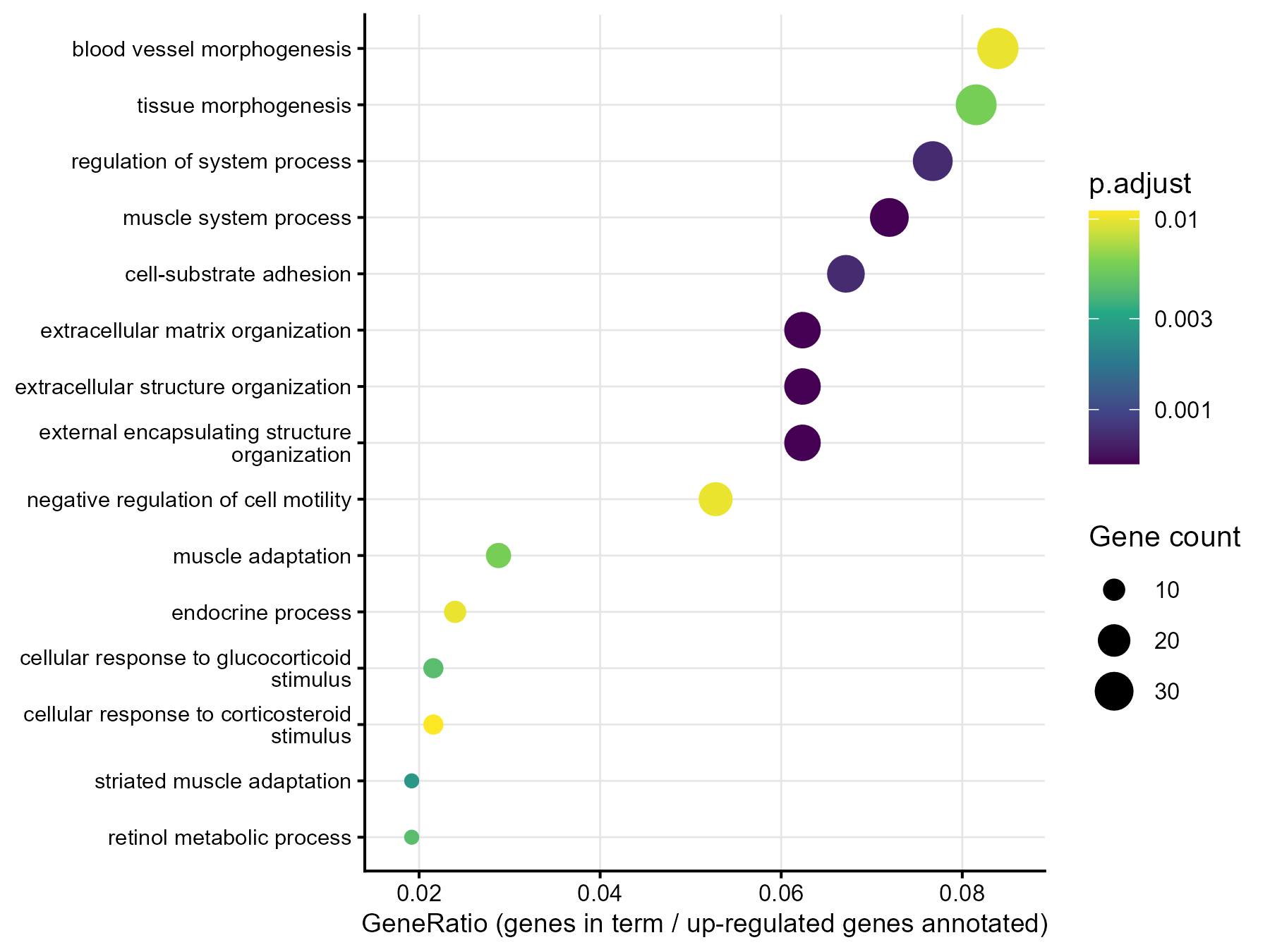
展示差异基因的 GO 生物过程(BP)富集结果:横轴为 GeneRatio,点的大小为富集到该条目的基因数,颜色为校正后 P 值,一张图同时给出富集比例、基因数和显著性。
图与代码
code/R/main.R
suppressPackageStartupMessages(library(ggplot2))

d <- read.csv("data/go_top15.csv", encoding = "UTF-8")      # 已按 GeneRatio 从高到低排列(make_data.R)
d$label <- gsub("|", "\n", d$label, fixed = TRUE)
d$ID <- factor(d$ID, levels = rev(d$ID))                    # 第 1 行画在最上面
lab <- setNames(d$label, d$ID)

write.csv(data.frame(rank = seq_len(nrow(d)), id = as.character(d$ID), count = d$Count,
                     gene_ratio = sprintf("%.4f", d$gene_ratio), p_adjust = sprintf("%.3e", d$p.adjust)),
          "outputs/stats_r.csv", row.names = FALSE, quote = FALSE)

p <- ggplot(d, aes(gene_ratio, ID, size = Count, colour = p.adjust)) +
  geom_point() +
  scale_y_discrete(labels = lab) +
  scale_size_continuous(range = c(1.8, 6), breaks = c(10, 20, 30)) +
  scale_colour_viridis_c(trans = "log10", breaks = c(0.001, 0.003, 0.01), labels = c("0.001", "0.003", "0.01"),
                         guide = guide_colourbar(order = 1)) +
  scale_x_continuous(breaks = seq(0.02, 0.08, 0.02), expand = expansion(mult = c(0.08, 0.08))) +
  labs(x = "GeneRatio (genes in term / up-regulated genes annotated)", y = NULL, size = "Gene count", colour = "p.adjust") +
  theme_classic(base_size = 10) +
  theme(panel.grid.major = element_line(colour = "grey90", linewidth = 0.3),
        axis.text.y = element_text(size = 7.5, lineheight = 0.85), axis.title.x = element_text(size = 9))

ggsave("outputs/figure_r.png", p, width = 6, height = 4.5, dpi = 300, bg = "white")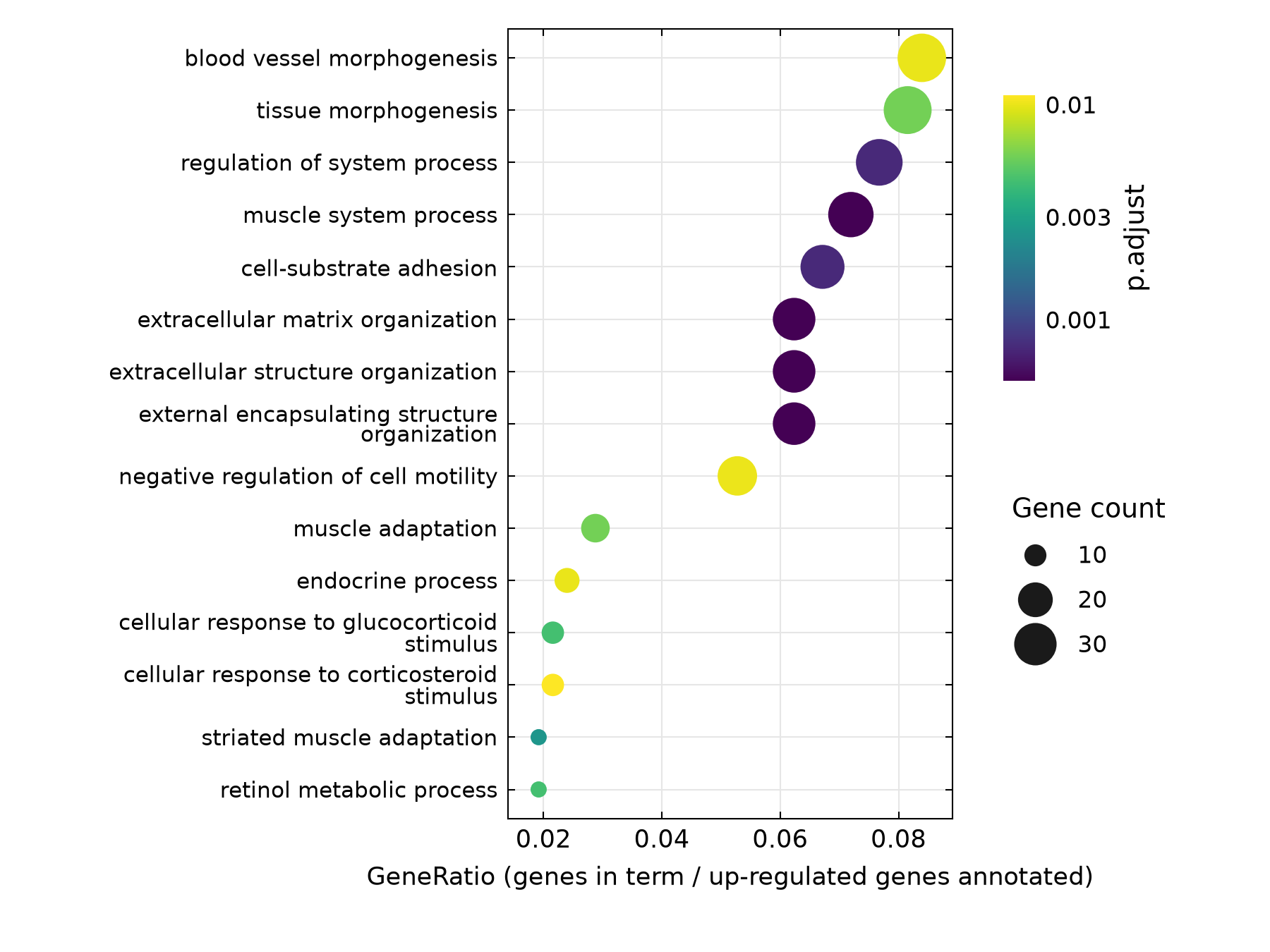
code/py/main.py
import numpy as np
import pandas as pd
import matplotlib.pyplot as plt
from matplotlib.colors import LogNorm
from matplotlib.lines import Line2D
import scienceplots  # noqa: F401

plt.style.use(["science", "no-latex"])
plt.rcParams["font.family"] = "sans-serif"
plt.rcParams["savefig.bbox"] = "standard"                      # scienceplots 默认裁白边,这里保持 6×4.5 in 画布

d = pd.read_csv("data/go_top15.csv")                          # 已按 GeneRatio 从高到低排列(make_data.R)
d["label"] = d["label"].str.replace("|", "\n", regex=False)
n = len(d)

pd.DataFrame({"rank": range(1, n + 1), "id": d["ID"], "count": d["Count"],
              "gene_ratio": [f"{v:.4f}" for v in d.gene_ratio], "p_adjust": [f"{v:.3e}" for v in d["p.adjust"]]}
             ).to_csv("outputs/stats_py.csv", index=False)

cmin, cmax = d.Count.min(), d.Count.max()
def diam(c):                                                   # 与 R 的 scale_size 相同:直径 = 下限 + 系数 × √(缩放到 0~1 的计数)
    return 4.5 + 11 * np.sqrt((np.asarray(c, float) - cmin) / (cmax - cmin))

fig, ax = plt.subplots(figsize=(6, 4.5))
fig.set_layout_engine("none")
fig.subplots_adjust(left=0.40, right=0.75, bottom=0.14, top=0.97)
y = np.arange(n)[::-1]                                         # 第 1 行画在最上面
sc = ax.scatter(d.gene_ratio, y, s=diam(d.Count) ** 2, c=d["p.adjust"], cmap="viridis",
                norm=LogNorm(vmin=d["p.adjust"].min(), vmax=d["p.adjust"].max()), zorder=3)
ax.set_yticks(y, d["label"], fontsize=7.5, linespacing=0.9)
ax.grid(True, color="#E6E6E6", lw=0.5, zorder=0)
ax.set_axisbelow(True)
ax.margins(x=0.08, y=0.04)
ax.set_xlabel("GeneRatio (genes in term / up-regulated genes annotated)", fontsize=8.5)
ax.tick_params(which="both", length=2.5)
ax.tick_params(axis="x", labelsize=8.5)
ax.tick_params(which="minor", length=0)

cax = fig.add_axes([0.79, 0.60, 0.025, 0.30])
cb = fig.colorbar(sc, cax=cax)
cb.set_ticks([0.001, 0.003, 0.01], labels=["0.001", "0.003", "0.01"])
cb.ax.minorticks_off()
cb.set_label("p.adjust", fontsize=9)
cb.outline.set_visible(False)
cb.ax.tick_params(length=0, labelsize=8)

handles = [Line2D([], [], marker="o", ls="", ms=float(diam(c)), mfc="#1A1A1A", mec="none", label=str(c)) for c in (10, 20, 30)]
fig.legend(handles=handles, title="Gene count", loc="upper left", bbox_to_anchor=(0.78, 0.50), frameon=False,
           fontsize=8, title_fontsize=9, labelspacing=0.9, alignment="left")
fig.savefig("outputs/figure_py.png", dpi=300, facecolor="white")
什么时候用
- 差异基因的过表达分析(ORA)之后,概览显著富集的功能条目
- 同时比较多个条目的基因数、占比和显著程度
- 作为论文或汇报中富集结果的标准展示
常见误用
- 结果依赖背景基因集的定义(本例取有 padj 的 17,896 个基因,enrichGO 再与 GO BP 注释取交集,实际参与检验的背景为 12,332 个,即 BgRatio 的分母)和差异基因的阈值;换背景或阈值,条目和 P 值都会变
- GO 条目有层级和包含关系,高度冗余:本图中 extracellular matrix organization、extracellular structure organization、external encapsulating structure organization 三条的基因集几乎相同,是同一信号的重复展示;本例没有做去冗余(simplify)
- GeneRatio 高不等于富集更显著,也不等于富集倍数更高;条目按 GeneRatio 排列,不是按 p.adjust 排列。这里展示的是 p.adjust 最小的 15 条,其 p.adjust 在 0.0005~0.011 之间
- 富集是统计关联,不能说明这些通路被“激活”或有因果作用;GO 注释随版本更新,结果会随版本变化,需记录版本
数据与下载
数据:R/Bioconductor 数据包 airway(人气道平滑肌细胞,地塞米松处理 vs 未处理,4 个细胞系各 1 对,共 8 个样本)+ Gene Ontology 注释(GO.db 3.22.0,org.Hs.eg.db 3.22.0,GO 数据日期 2025-07-22)(airway 数据包(Bioconductor,LGPL);原始数据来自 GEO GSE52778,原文 Himes et al. 2014(PLoS ONE,CC BY);Gene Ontology(CC BY 4.0);GO.db、org.Hs.eg.db、clusterProfiler 为 Bioconductor 软件包(Artistic-2.0))。差异分析为 DESeq2(~ cell + dex,参考水平 untrt,BH 校正,未收缩 LFC)。上调基因 = padj < 0.05 且 log2FC > 1(528 个,其中 417 个有 GO BP 注释);背景 = 有 padj 的 17,896 个基因,其中有 GO BP 注释、实际参与检验的 12,332 个(BgRatio 分母,见 data/versions.csv 的 n_background_annotated);clusterProfiler 4.18.4 的 enrichGO(BP,Ensembl ID,BH 校正,条目大小 10~500,未去冗余)共检验 3,710 个条目,p.adjust < 0.05 的 96 个,图中为 p.adjust 最小的 15 个。版本:DESeq2 1.50.2,airway 1.30.0,clusterProfiler 4.18.4,GO.db 3.22.0,org.Hs.eg.db 3.22.0(data/versions.csv)。
下载包 sha256:3d3f5d8f32bde4061b19c131301e3f181be44c5a37a57599e14554bb3626359f