差异基因表达热图（行标准化 + 层次聚类）

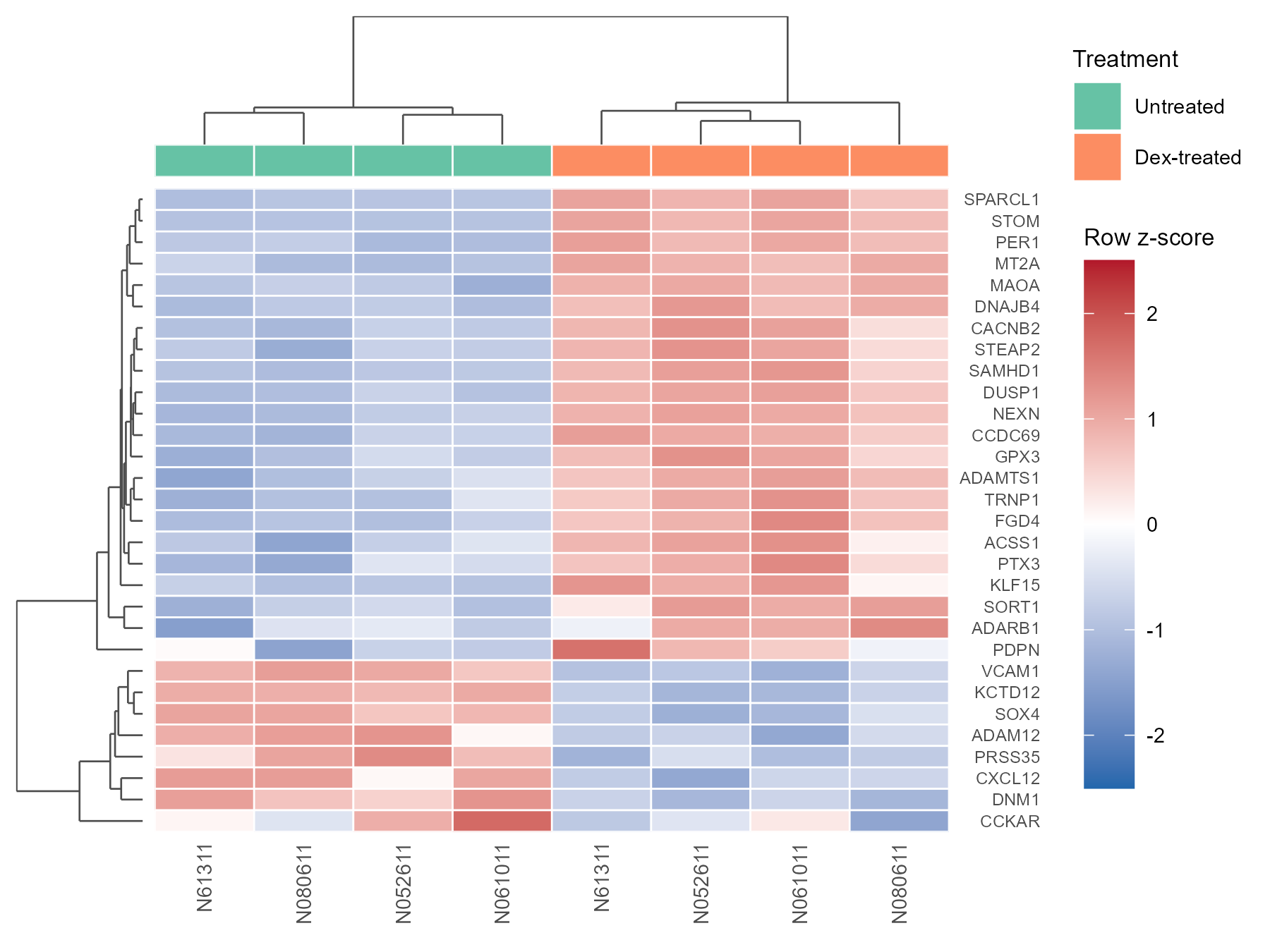
用颜色展示 30 个差异基因在 8 个样本中的相对表达（按基因标准化为 z 分数），并对基因和样本做层次聚类，直观看出表达模式相似的基因与样本分组。

图与代码

code/R/main.R

suppressPackageStartupMessages({ library(ggplot2); library(patchwork) })

res <- read.csv("data/deg_results.csv", encoding = "UTF-8")
vst <- read.csv("data/deg_vst.csv", encoding = "UTF-8", check.names = FALSE)
sm <- read.csv("data/samples.csv", encoding = "UTF-8")

# 前 30 个差异基因：padj 最小（同值按 gene_id），矩阵为 DESeq2 vst 值
top <- head(res[order(res$padj, res$gene_id, method = "radix"), ], 30)
m <- as.matrix(vst[match(top$gene_id, vst$gene_id), sm$sample])
rownames(m) <- top$symbol
z <- t(scale(t(m)))                                         # 行标准化：每个基因 8 个样本的 z 分数（样本标准差，n-1）

# 层次聚类：欧氏距离 + 平均连接；叶序规则（R 与 Python 共用）：每次合并处，含原始序号更小叶子的分支在前
hc_r <- hclust(dist(z), method = "average")
hc_c <- hclust(dist(t(z)), method = "average")
dend <- function(hc) {
  mg <- hc$merge; n <- nrow(mg) + 1
  ord <- function(k) {
    ch <- lapply(mg[k, ], function(i) if (i < 0) -i else ord(i))
    if (min(ch[[1]]) > min(ch[[2]])) ch <- rev(ch)
    c(ch[[1]], ch[[2]])
  }
  order <- ord(n - 1); rank <- match(seq_len(n), order)
  segs <- list()
  node <- function(k) {                                      # 返回 list(x, h)
    ch <- lapply(mg[k, ], function(i) if (i < 0) list(x = rank[-i], h = 0) else node(i))
    if (ch[[1]]$x > ch[[2]]$x) ch <- rev(ch)
    h <- hc$height[k]
    segs[[length(segs) + 1]] <<- data.frame(x = c(ch[[1]]$x, ch[[2]]$x, ch[[1]]$x), xend = c(ch[[1]]$x, ch[[2]]$x, ch[[2]]$x),
                                            h = c(ch[[1]]$h, ch[[2]]$h, h), hend = c(h, h, h))
    list(x = (ch[[1]]$x + ch[[2]]$x) / 2, h = h)
  }
  node(n - 1)
  list(order = order, segs = do.call(rbind, segs))
}
dr <- dend(hc_r); dc <- dend(hc_c)
ng <- nrow(z); ns <- ncol(z)

st <- data.frame(item = c(paste0("row_", seq_len(ng)), paste0("col_", seq_len(ns))),
                 value = c(rownames(z)[dr$order], colnames(z)[dc$order]))
write.csv(st, "outputs/stats_r.csv", row.names = FALSE, quote = FALSE)

# 热图数据（行：叶序第 1 个在最上；列：叶序第 1 个在最左）
g <- expand.grid(r = seq_len(ng), c = seq_len(ns))
g$z <- mapply(function(i, j) z[dr$order[i], dc$order[j]], g$r, g$c)
g$y <- ng + 1 - g$r
cell <- sm$cell[match(colnames(z)[dc$order], sm$sample)]
dex <- sm$dex[match(colnames(z)[dc$order], sm$sample)]

xs <- scale_x_continuous(limits = c(0.5, ns + 0.5), expand = c(0, 0))
p_heat <- ggplot(g, aes(c, y, fill = z)) +
  geom_tile(colour = "white", linewidth = 0.3) +
  scale_fill_gradient2(low = "#2166AC", mid = "white", high = "#B2182B", midpoint = 0, limits = c(-2.5, 2.5),
                       breaks = c(-2, -1, 0, 1, 2), name = "Row z-score") +
  scale_x_continuous(breaks = seq_len(ns), labels = cell, limits = c(0.5, ns + 0.5), expand = c(0, 0)) +
  scale_y_continuous(breaks = ng + 1 - seq_len(ng), labels = rownames(z)[dr$order], limits = c(0.5, ng + 0.5),
                     expand = c(0, 0), position = "right") +
  labs(x = NULL, y = NULL) +
  theme_minimal(base_size = 8) +
  theme(panel.grid = element_blank(), axis.text.x = element_text(angle = 90, hjust = 1, vjust = 0.5, size = 7),
        axis.text.y = element_text(size = 5.8), legend.key.height = unit(0.5, "in"),
        legend.title = element_text(size = 8), legend.text = element_text(size = 7))

p_dex <- ggplot(data.frame(x = seq_len(ns), dex = factor(dex, levels = c("untrt", "trt"))), aes(x, 1, fill = dex)) +
  geom_tile(colour = "white", linewidth = 0.3) +
  scale_fill_manual(values = c(untrt = "#66C2A5", trt = "#FC8D62"), labels = c("Untreated", "Dex-treated"), name = "Treatment") +
  xs + scale_y_continuous(expand = c(0, 0)) + theme_void(base_size = 8) +
  theme(legend.title = element_text(size = 8), legend.text = element_text(size = 7))

p_col <- ggplot(dc$segs, aes(x, h, xend = xend, yend = hend)) + geom_segment(linewidth = 0.3, colour = "grey30") +
  xs + scale_y_continuous(expand = c(0, 0.02)) + theme_void()
p_row <- ggplot(dr$segs, aes(h, ng + 1 - x, xend = hend, yend = ng + 1 - xend)) +
  geom_segment(aes(x = h, y = ng + 1 - x, xend = hend, yend = ng + 1 - xend), linewidth = 0.3, colour = "grey30") +
  scale_x_reverse(expand = c(0, 0.02)) + scale_y_continuous(limits = c(0.5, ng + 0.5), expand = c(0, 0)) + theme_void()

design <- "#A\n#B\nCD"
p <- p_col + p_dex + p_row + p_heat +
  plot_layout(design = design, widths = c(0.16, 1), heights = c(0.2, 0.05, 1), guides = "collect")

ggsave("outputs/figure_r.png", p, width = 6, height = 4.5, dpi = 300, bg = "white")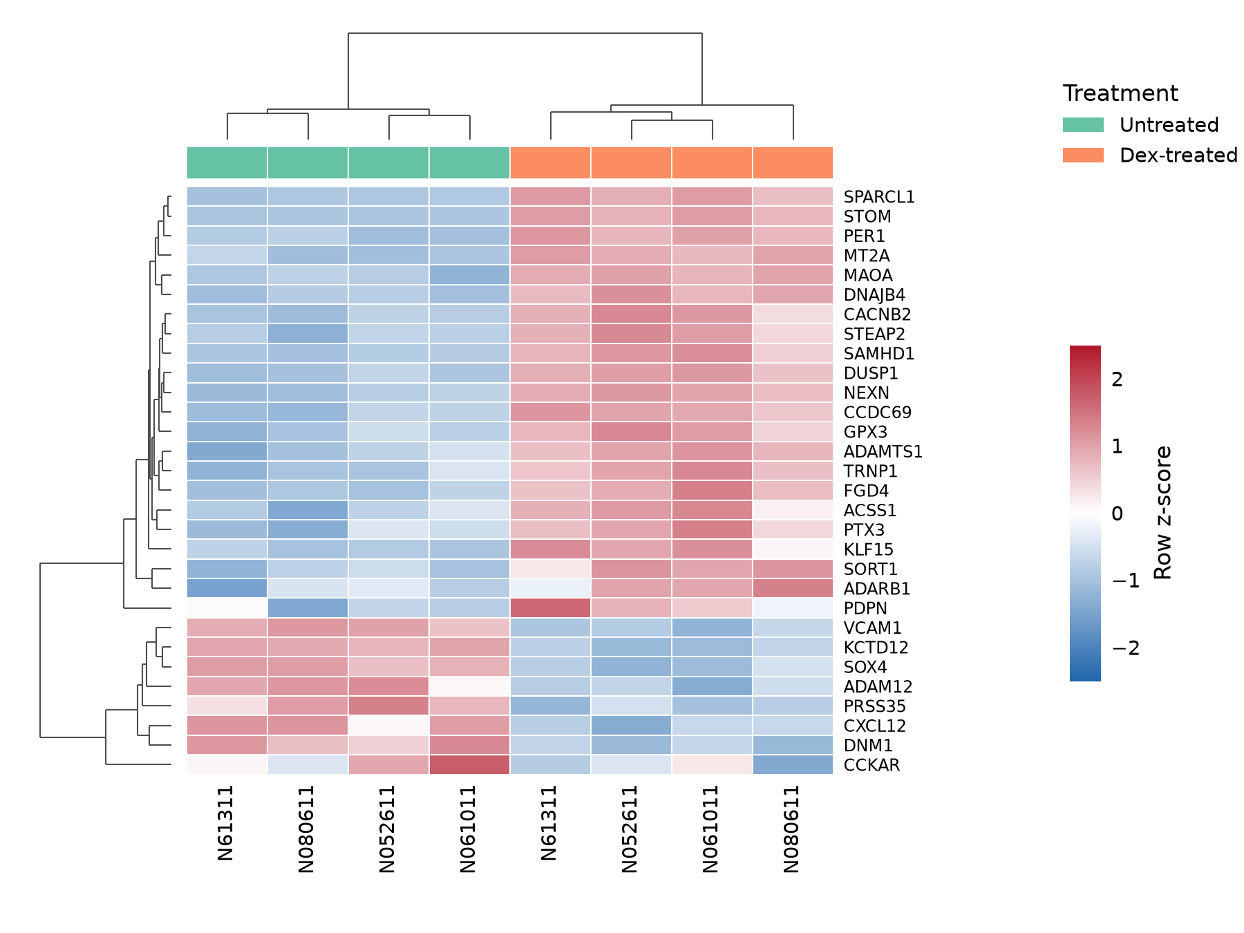

code/py/main.py

import numpy as np
import pandas as pd
import matplotlib.pyplot as plt
from matplotlib.colors import LinearSegmentedColormap
from matplotlib.patches import Patch
from scipy.cluster.hierarchy import linkage
import scienceplots  # noqa: F401

plt.style.use(["science", "no-latex"])
plt.rcParams["font.family"] = "sans-serif"
plt.rcParams["savefig.bbox"] = "standard"                      # scienceplots 默认裁白边，这里保持 6×4.5 in 画布

res = pd.read_csv("data/deg_results.csv")
vst = pd.read_csv("data/deg_vst.csv").set_index("gene_id")
sm = pd.read_csv("data/samples.csv")

# 前 30 个差异基因：padj 最小（同值按 gene_id），矩阵为 DESeq2 vst 值
top = res.sort_values(["padj", "gene_id"]).head(30)
m = vst.loc[top.gene_id, sm["sample"]].to_numpy()
syms = list(top.symbol)
z = (m - m.mean(axis=1, keepdims=True)) / m.std(axis=1, ddof=1, keepdims=True)    # 行标准化（样本标准差，n-1）

# 层次聚类：欧氏距离 + 平均连接；叶序规则（R 与 Python 共用）：每次合并处，含原始序号更小叶子的分支在前
Zr = linkage(z, method="average", metric="euclidean")
Zc = linkage(z.T, method="average", metric="euclidean")


def dend(Z):
    n = Z.shape[0] + 1

    def order(k):
        ch = [order(int(i) - n) if i >= n else [int(i)] for i in Z[k, :2]]
        if min(ch[0]) > min(ch[1]):
            ch = ch[::-1]
        return ch[0] + ch[1]

    od = order(n - 2)
    rank = {leaf: i + 1 for i, leaf in enumerate(od)}
    segs = []

    def node(k):
        ch = [node(int(i) - n) if i >= n else (rank[int(i)], 0.0) for i in Z[k, :2]]
        if ch[0][0] > ch[1][0]:
            ch = ch[::-1]
        h = Z[k, 2]
        (x1, h1), (x2, h2) = ch
        segs.extend([(x1, h1, x1, h), (x2, h2, x2, h), (x1, h, x2, h)])
        return (x1 + x2) / 2, h

    node(n - 2)
    return od, segs


ro, rsegs = dend(Zr)
co, csegs = dend(Zc)
ng, ns = z.shape
cols = list(sm["sample"])

st = pd.DataFrame({"item": [f"row_{i}" for i in range(1, ng + 1)] + [f"col_{j}" for j in range(1, ns + 1)],
                   "value": [syms[i] for i in ro] + [cols[j] for j in co]})
st.to_csv("outputs/stats_py.csv", index=False)

zo = z[np.ix_(ro, co)]
cell = [sm["cell"][j] for j in co]
dex = [sm["dex"][j] for j in co]
dex_col = {"untrt": "#66C2A5", "trt": "#FC8D62"}
cmap = LinearSegmentedColormap.from_list("bwr_clean", ["#2166AC", "#FFFFFF", "#B2182B"])

fig = plt.figure(figsize=(6, 4.5))
L, B, W, H = 0.15, 0.17, 0.52, 0.63                     # 热图区（图幅比例）
ax = fig.add_axes([L, B, W, H])
im = ax.pcolormesh(zo, cmap=cmap, vmin=-2.5, vmax=2.5, edgecolors="white", linewidth=0.4)
ax.set_xlim(0, ns)
ax.set_ylim(ng, 0)
ax.set_xticks(np.arange(ns) + 0.5, cell, rotation=90, fontsize=7)
ax.yaxis.tick_right()
ax.set_yticks(np.arange(ng) + 0.5, [syms[i] for i in ro], fontsize=5.8)
ax.tick_params(which="both", length=0)
for s in ax.spines.values():
    s.set_visible(False)

axs = fig.add_axes([L, B + H + 0.008, W, 0.035])        # 处理分组色条
axs.pcolormesh(np.arange(ns + 1), [0, 1], np.zeros((1, ns)), cmap="Greys", alpha=0)
for j, d in enumerate(dex):
    axs.add_patch(plt.Rectangle((j, 0), 1, 1, fc=dex_col[d], ec="white", lw=0.4))
axs.set_xlim(0, ns)
axs.set_ylim(0, 1)
axs.axis("off")

axc = fig.add_axes([L, B + H + 0.05, W, 0.12])          # 列树
for x1, h1, x2, h2 in csegs:
    axc.plot([x1 - 0.5, x2 - 0.5], [h1, h2], c="#4D4D4D", lw=0.5, solid_capstyle="butt")
axc.set_xlim(0, ns)
axc.set_ylim(0, None)
axc.margins(y=0.02)
axc.axis("off")

axr = fig.add_axes([0.03, B, 0.11, H])                  # 行树（根在左）
for x1, h1, x2, h2 in rsegs:
    axr.plot([h1, h2], [x1 - 0.5, x2 - 0.5], c="#4D4D4D", lw=0.5, solid_capstyle="butt")
axr.set_ylim(ng, 0)
axr.invert_xaxis()
axr.margins(x=0.02)
axr.axis("off")

cax = fig.add_axes([0.86, 0.27, 0.025, 0.36])
cb = fig.colorbar(im, cax=cax, ticks=[-2, -1, 0, 1, 2])
cb.set_label("Row z-score", fontsize=8)
cb.outline.set_visible(False)
cb.ax.tick_params(which="both", length=0, labelsize=7)
fig.legend(handles=[Patch(fc=dex_col["untrt"], label="Untreated"), Patch(fc=dex_col["trt"], label="Dex-treated")],
           title="Treatment", loc="upper left", bbox_to_anchor=(0.84, 0.93), frameon=False, fontsize=7, title_fontsize=8,
           alignment="left")
fig.savefig("outputs/figure_py.png", dpi=300, facecolor="white")

什么时候用

展示一组候选基因（如差异基因）在各样本中的表达模式
检查样本是否按处理或批次聚在一起
找出表达趋势相同的基因模块

常见误用

行标准化（z 分数）去掉了基因的绝对表达水平，只保留各样本间的相对高低；颜色深浅不能跨基因比较表达量
这 30 个基因是用同一批数据按显著性挑出来的，所以样本按处理分开几乎是必然的，不能当作处理有效的独立证据
聚类结果取决于距离和连接方式（本例欧氏距离 + 平均连接）及所选基因；叶子的左右顺序可以任意翻转，不含信息
本例只有 8 个样本，z 分数的范围受样本数限制；不同细胞系是配对设计的，热图没有去除细胞系效应

数据与下载

数据：R/Bioconductor 数据包 airway（人气道平滑肌细胞，地塞米松处理 vs 未处理，4 个细胞系各 1 对，共 8 个样本）（airway 数据包（Bioconductor，LGPL）；原始数据来自 GEO GSE52778，原文 Himes et al. 2014（PLoS ONE，CC BY）；基因注释来自 org.Hs.eg.db（Artistic-2.0））。先做 DESeq2 差异分析（~ cell + dex，参考水平 untrt，BH 校正），取 padj < 0.05 且 |log2FC| > 1 的基因中 padj 最小的 30 个；表达值为 vst（方差稳定变换，blind = FALSE）矩阵，对每个基因做 z 分数（样本标准差，n−1）。行、列均用欧氏距离 + 平均连接聚类；叶序规则为每次合并处含原始序号较小叶子的分支在前，R 与 Python 两版聚类顺序一致（outputs/stats_*.csv 可核对）。

下载 R / Python 代码与数据（794 KB）

下载包 sha256：3460b9d9f7dde68f9ed898e0675e94bc9dca417cc6f02ebd3b97175b828d5d59

图与代码

什么时候用

常见误用

数据与下载

相关顶刊复刻