MA 图(平均表达 vs 倍数变化)
GAL-0013
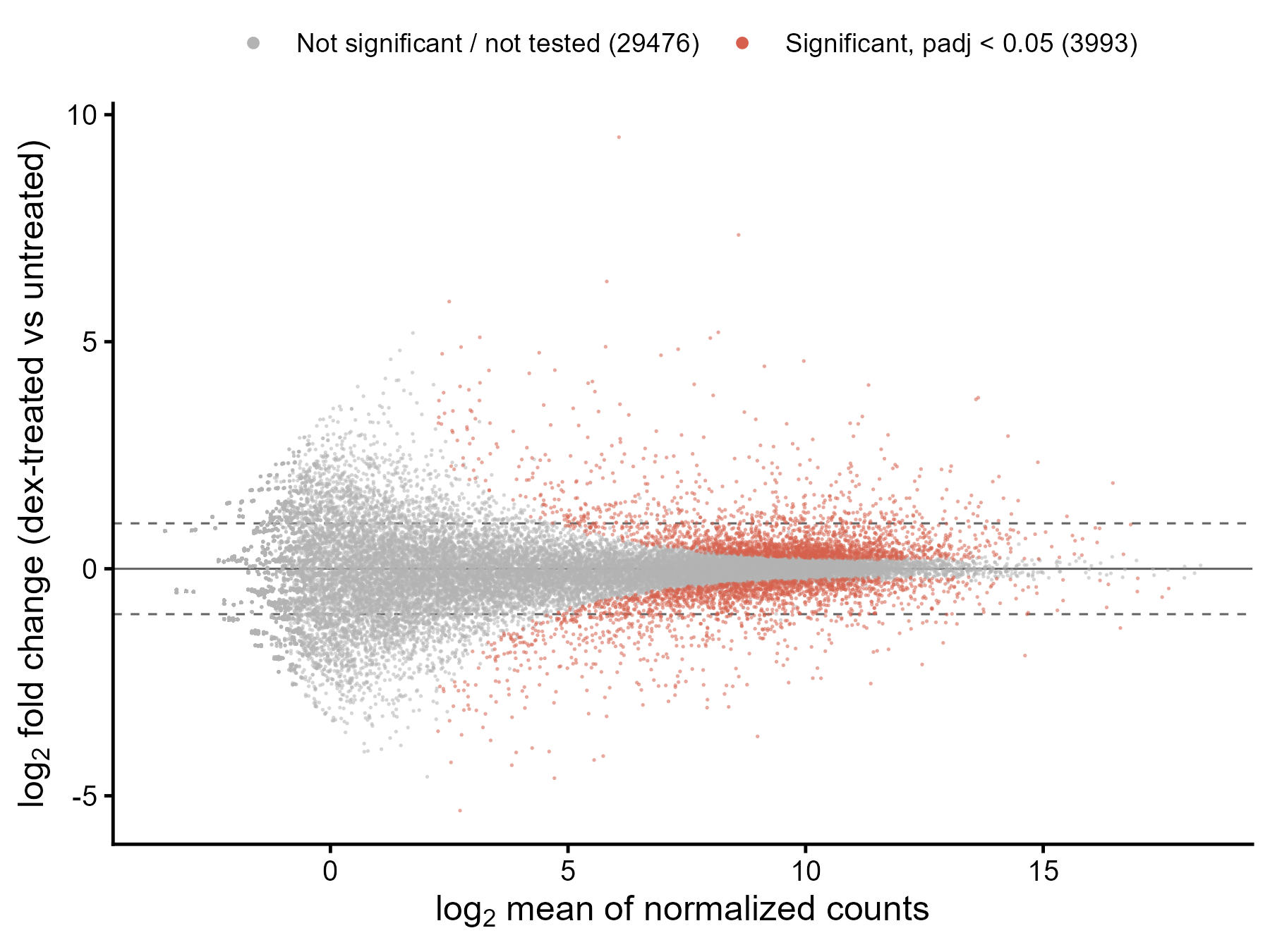
横轴是基因的平均表达量(log2),纵轴是 log2 倍数变化,用来检查差异表达结果与表达量的关系,并看显著基因分布在哪些表达水平。
图与代码
code/R/main.R
suppressPackageStartupMessages(library(ggplot2))

d <- read.csv("data/deseq_results.csv", encoding = "UTF-8")
d$x <- log2(d$baseMean)                                    # baseMean:各样本标准化计数的均值(全零行已在 DESeq2 前删除)
d$grp <- ifelse(!is.na(d$padj) & d$padj < 0.05, "Significant (padj < 0.05)", "Not significant / not tested")
d$grp <- factor(d$grp, levels = c("Not significant / not tested", "Significant (padj < 0.05)"))
d <- d[order(d$grp), ]                                     # 显著基因最后画,压在上层

cnt <- table(d$grp)
st <- data.frame(item = c("n_genes", "n_significant", "n_not_significant_or_not_tested", "n_padj_na"),
                 value = c(nrow(d), as.integer(cnt[2]), as.integer(cnt[1]), sum(is.na(d$padj))))
write.csv(st, "outputs/stats_r.csv", row.names = FALSE, quote = FALSE)

p <- ggplot(d, aes(x, log2FoldChange, colour = grp)) +
  geom_hline(yintercept = c(-1, 1), linetype = "dashed", linewidth = 0.35, colour = "grey40") +
  geom_hline(yintercept = 0, linewidth = 0.35, colour = "grey40") +
  geom_point(size = 0.6, alpha = 0.55, stroke = 0) +
  scale_colour_manual(values = c("Not significant / not tested" = "grey70", "Significant (padj < 0.05)" = "#D6604D"),
                      labels = c(paste0("Not significant / not tested (", cnt[1], ")"), paste0("Significant, padj < 0.05 (", cnt[2], ")"))) +
  guides(colour = guide_legend(override.aes = list(size = 2, alpha = 1))) +
  labs(x = expression(log[2]~"mean of normalized counts"), y = expression(log[2]~"fold change (dex-treated vs untreated)"), colour = NULL) +
  theme_classic(base_size = 12) +
  theme(legend.position = "top", legend.margin = margin(0, 0, 0, 0), legend.text = element_text(size = 9))

ggsave("outputs/figure_r.png", p, width = 6, height = 4.5, dpi = 300, bg = "white")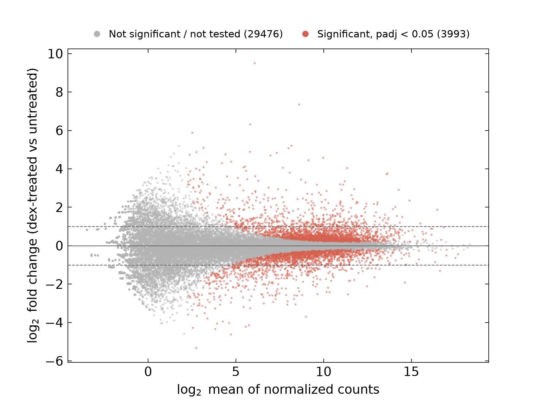
code/py/main.py
import numpy as np
import pandas as pd
import matplotlib.pyplot as plt
from matplotlib.lines import Line2D
import scienceplots  # noqa: F401

plt.style.use(["science", "no-latex"])
plt.rcParams["font.family"] = "sans-serif"
plt.rcParams["savefig.bbox"] = "standard"                      # scienceplots 默认裁白边,这里保持 6×4.5 in 画布
plt.rcParams["mathtext.fontset"] = "dejavusans"

d = pd.read_csv("data/deseq_results.csv")
d["x"] = np.log2(d["baseMean"])                              # baseMean:各样本标准化计数的均值(全零行已在 DESeq2 前删除)
sig = d["padj"].notna() & (d["padj"] < 0.05)
n_sig, n_ns = int(sig.sum()), int((~sig).sum())

st = pd.DataFrame({"item": ["n_genes", "n_significant", "n_not_significant_or_not_tested", "n_padj_na"],
                   "value": [len(d), n_sig, n_ns, int(d["padj"].isna().sum())]})
st.to_csv("outputs/stats_py.csv", index=False)

c_ns, c_sig = "#B3B3B3", "#D6604D"
fig, ax = plt.subplots(figsize=(6, 4.5))
ax.axhline(0, lw=0.6, c="#666666")
for v in (-1, 1):
    ax.axhline(v, ls="--", lw=0.6, c="#666666")
ax.scatter(d.x[~sig], d.log2FoldChange[~sig], s=2.5, c=c_ns, alpha=0.55, linewidths=0)
ax.scatter(d.x[sig], d.log2FoldChange[sig], s=2.5, c=c_sig, alpha=0.55, linewidths=0)
ax.set_xlabel(r"$\log_2$ mean of normalized counts")
ax.set_ylabel(r"$\log_2$ fold change (dex-treated vs untreated)")
ax.tick_params(which="minor", length=0)
handles = [Line2D([], [], marker="o", ls="", ms=4, c=c_ns, label=f"Not significant / not tested ({n_ns})"),
           Line2D([], [], marker="o", ls="", ms=4, c=c_sig, label=f"Significant, padj < 0.05 ({n_sig})")]
ax.legend(handles=handles, loc="lower center", bbox_to_anchor=(0.5, 1.0), ncol=2, frameon=False,
          handletextpad=0.2, columnspacing=1.2, fontsize=8)
fig.savefig("outputs/figure_py.png", dpi=300, facecolor="white")
什么时候用
- 差异分析后检查标准化是否合理(点云应大致围绕 0 对称)
- 观察倍数变化的离散程度如何随表达量变化(低表达基因更分散)
- 配合火山图,说明显著基因的表达量范围
常见误用
- 本例的 log2FC 是 DESeq2 的最大似然估计,没有做 LFC 收缩(lfcShrink);低表达基因的 log2FC 方差大,图左侧呈喇叭口状,其中很大的倍数变化多是噪声。做收缩后再画,低表达基因的点会向 0 靠拢
- 灰色点包括“padj ≥ 0.05”和“padj 为 NA(低表达被独立过滤或被判为离群值)”两类,图中没有区分
- 这里“显著”只按 padj < 0.05 着色,没有加 |log2FC| 阈值,所以 0 附近也有显著基因(高表达基因的小幅变化也能显著)
- 横轴是 DESeq2 的 baseMean(各样本标准化计数的均值)取 log2,不是 RPKM/TPM
数据与下载
数据:R/Bioconductor 数据包 airway(人气道平滑肌细胞,地塞米松处理 vs 未处理,4 个细胞系各 1 对,共 8 个样本)(airway 数据包(Bioconductor,LGPL);原始数据来自 GEO GSE52778,原文 Himes et al. 2014(PLoS ONE,CC BY);基因注释来自 org.Hs.eg.db(Artistic-2.0))。DESeq2 差异分析(~ cell + dex,参考水平 untrt,BH 校正,未收缩 LFC)。图中为删除全零基因后的 33,469 个基因,其中 padj < 0.05 的 3,993 个着色;图中 log2FC = ±1 的两条虚线只是参考线(对应火山图的倍数阈值),不参与着色。统计只在 R 端计算一次(code/R/make_data.R),两版作图脚本读同一份结果 CSV。
下载包 sha256:b91754c0b951c7cc85e79cf8d183c280ee42fc0ecadab9bcf026864bc301eed3