校准曲线(按预测概率十分位分组)
GAL-0009
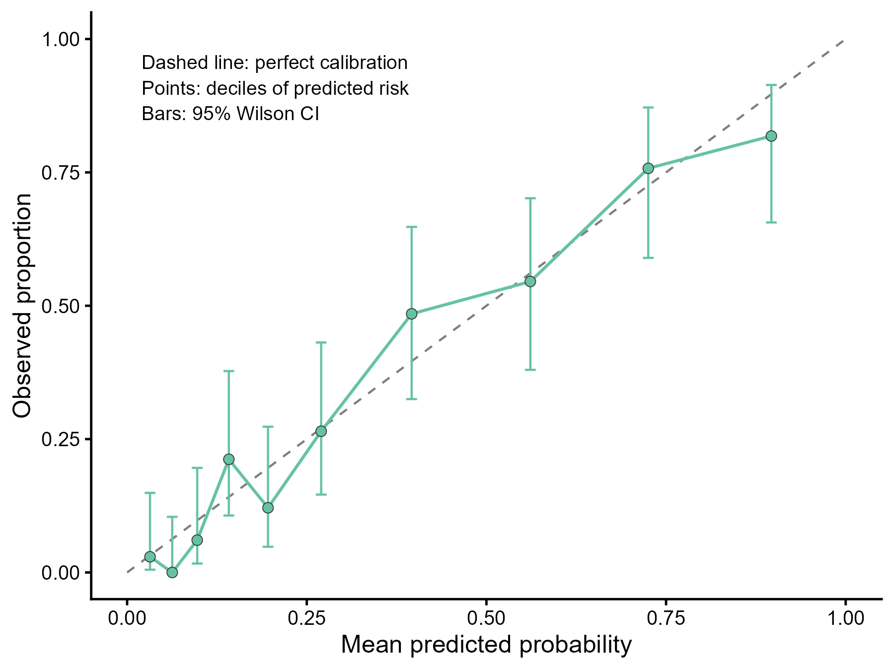
把测试集样本按模型预测概率从低到高分成十组,比较每组的平均预测概率与实际观察到的事件比例,并与理想的对角线对照,检查预测概率是否“准”。
图与代码
code/R/main.R
suppressPackageStartupMessages(library(ggplot2))

tr <- read.csv("data/pima_tr.csv", encoding = "UTF-8")
te <- read.csv("data/pima_te.csv", encoding = "UTF-8")
tr$y <- as.integer(tr$type == "Yes")
te$y <- as.integer(te$type == "Yes")

# 训练集上拟合逻辑回归,在测试集上做分组校准
m <- glm(y ~ glu + bmi + age + ped, family = binomial, data = tr)
te$pred <- predict(m, newdata = te, type = "response")

# 按预测概率排序后等分为 10 组(并列时按原顺序)
n <- nrow(te)
ord <- order(te$pred)
te$decile <- NA_integer_
te$decile[ord] <- floor((seq_len(n) - 1) * 10 / n) + 1

z <- qnorm(0.975)
g <- do.call(rbind, lapply(1:10, function(k) {
  x <- te[te$decile == k, ]
  nk <- nrow(x); p <- mean(x$y)
  half <- z * sqrt(p * (1 - p) / nk + z^2 / (4 * nk^2)) / (1 + z^2 / nk)   # Wilson 95% 置信区间
  ctr <- (p + z^2 / (2 * nk)) / (1 + z^2 / nk)
  data.frame(decile = k, n = nk, mean_pred = mean(x$pred), events = sum(x$y), obs = p, lo = ctr - half, hi = ctr + half)
}))
write.csv(g, "outputs/stats_r.csv", row.names = FALSE)

p <- ggplot(g, aes(mean_pred, obs)) +
  annotate("segment", x = 0, y = 0, xend = 1, yend = 1, linetype = "dashed", colour = "grey50", linewidth = 0.5) +
  geom_errorbar(aes(ymin = lo, ymax = hi), width = 0.015, colour = "#66C2A5", linewidth = 0.5) +
  geom_line(colour = "#66C2A5", linewidth = 0.7) +
  geom_point(size = 2.2, shape = 21, fill = "#66C2A5", colour = "grey20", stroke = 0.3) +
  annotate("text", x = 0.02, y = 0.97, hjust = 0, vjust = 1, size = 3.3, lineheight = 1.1,
           label = "Dashed line: perfect calibration\nPoints: deciles of predicted risk\nBars: 95% Wilson CI") +
  scale_x_continuous(limits = c(0, 1), breaks = seq(0, 1, 0.25)) +
  scale_y_continuous(limits = c(0, 1), breaks = seq(0, 1, 0.25)) +
  labs(x = "Mean predicted probability", y = "Observed proportion") +
  theme_classic(base_size = 12)

ggsave("outputs/figure_r.png", p, width = 6, height = 4.5, dpi = 300, bg = "white")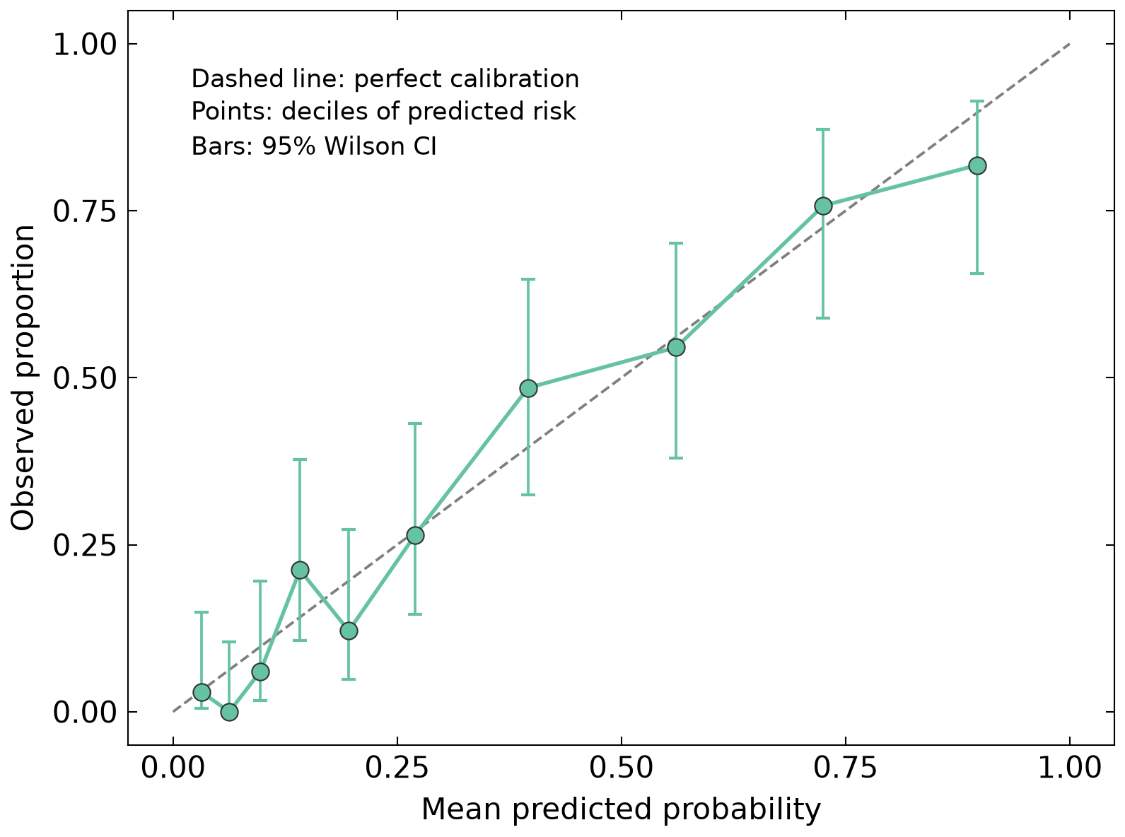
code/py/main.py
import numpy as np
import pandas as pd
import matplotlib.pyplot as plt
import scienceplots  # noqa: F401
import statsmodels.api as sm

plt.style.use(["science", "no-latex"])
plt.rcParams["font.family"] = "sans-serif"

tr = pd.read_csv("data/pima_tr.csv")
te = pd.read_csv("data/pima_te.csv")
tr["y"] = (tr["type"] == "Yes").astype(int)
te["y"] = (te["type"] == "Yes").astype(int)

# 训练集上拟合逻辑回归,在测试集上做分组校准
xs = ["glu", "bmi", "age", "ped"]
m = sm.Logit(tr["y"], sm.add_constant(tr[xs])).fit(disp=0)
te["pred"] = m.predict(sm.add_constant(te[xs])).to_numpy()

# 按预测概率排序后等分为 10 组(并列时按原顺序)
n = len(te)
ord_ = np.argsort(te["pred"].to_numpy(), kind="stable")
decile = np.empty(n, dtype=int)
decile[ord_] = (np.arange(n) * 10) // n + 1
te["decile"] = decile

z = 1.959963984540054
rows = []
for k in range(1, 11):
    x = te[te["decile"] == k]
    nk, p = len(x), x["y"].mean()
    ctr = (p + z**2 / (2 * nk)) / (1 + z**2 / nk)
    half = z * np.sqrt(p * (1 - p) / nk + z**2 / (4 * nk**2)) / (1 + z**2 / nk)  # Wilson 95% 置信区间
    rows.append((k, nk, x["pred"].mean(), x["y"].sum(), p, ctr - half, ctr + half))
g = pd.DataFrame(rows, columns=["decile", "n", "mean_pred", "events", "obs", "lo", "hi"])
g.to_csv("outputs/stats_py.csv", index=False)

fig, ax = plt.subplots(figsize=(6, 4.5))
ax.plot([0, 1], [0, 1], linestyle="--", color="#7F7F7F", lw=0.9)
ax.errorbar(g["mean_pred"], g["obs"], yerr=[g["obs"] - g["lo"], g["hi"] - g["obs"]], fmt="none",
            ecolor="#66C2A5", elinewidth=0.9, capsize=2.5)
ax.plot(g["mean_pred"], g["obs"], color="#66C2A5", lw=1.3)
ax.scatter(g["mean_pred"], g["obs"], s=34, facecolor="#66C2A5", edgecolor="#333333", linewidth=0.5, zorder=3)
ax.text(0.02, 0.97, "Dashed line: perfect calibration\nPoints: deciles of predicted risk\nBars: 95% Wilson CI",
        ha="left", va="top", fontsize=8.5, linespacing=1.3)
ax.set_xlim(-0.05, 1.05)
ax.set_ylim(-0.05, 1.05)
ax.set_xticks(np.arange(0, 1.01, 0.25))
ax.set_yticks(np.arange(0, 1.01, 0.25))
ax.set_xlabel("Mean predicted probability")
ax.set_ylabel("Observed proportion")
ax.minorticks_off()
fig.savefig("outputs/figure_py.png", dpi=300, facecolor="white")
什么时候用
- 评价预测模型给出的概率与实际发生率是否一致(校准度,calibration)
- 与 ROC/AUC 搭配:AUC 看区分度,校准曲线看概率的准确性
- 在独立数据(外部或测试集)上检验模型是否高估或低估风险
常见误用
- 分组校准图依赖分组方式:组数与分组边界不同,图形可能明显不同;组数太多则每组样本少、点很不稳
- 本例每组仅约 33 例,观察比例的置信区间(Wilson 区间)很宽,点偏离对角线不一定代表真正的失准
- 图中把各组的点用折线连起来只是为了便于观看,折线不是拟合出来的校准曲线,不能在组与组之间插值解读
- 分组会损失信息,且图形不能给出统一的量化结论;常与校准截距、校准斜率、平滑校准曲线(如 loess)配合报告
- 校准良好不代表区分度好,反之亦然;这里只展示测试集上的校准,不能推广到其他人群
数据与下载
数据:R 包 MASS 内置数据集 Pima.tr(训练,200 例)与 Pima.te(测试,332 例)(R 包 MASS 随 CRAN 分发(GPL-2 | GPL-3))。在 Pima.tr 上用逻辑回归拟合 type(Yes = 糖尿病)~ glu + bmi + age + ped,对 Pima.te 的 332 例预测患病概率, 按预测概率排序后等分为 10 组(每组 33 或 34 例),每组计算平均预测概率与观察到的糖尿病比例(Wilson 95% 置信区间)。
下载包 sha256:d9a22a45bcdfceb0b77a3397123e9b847eb8851ba182854cd628ac2921aa1359