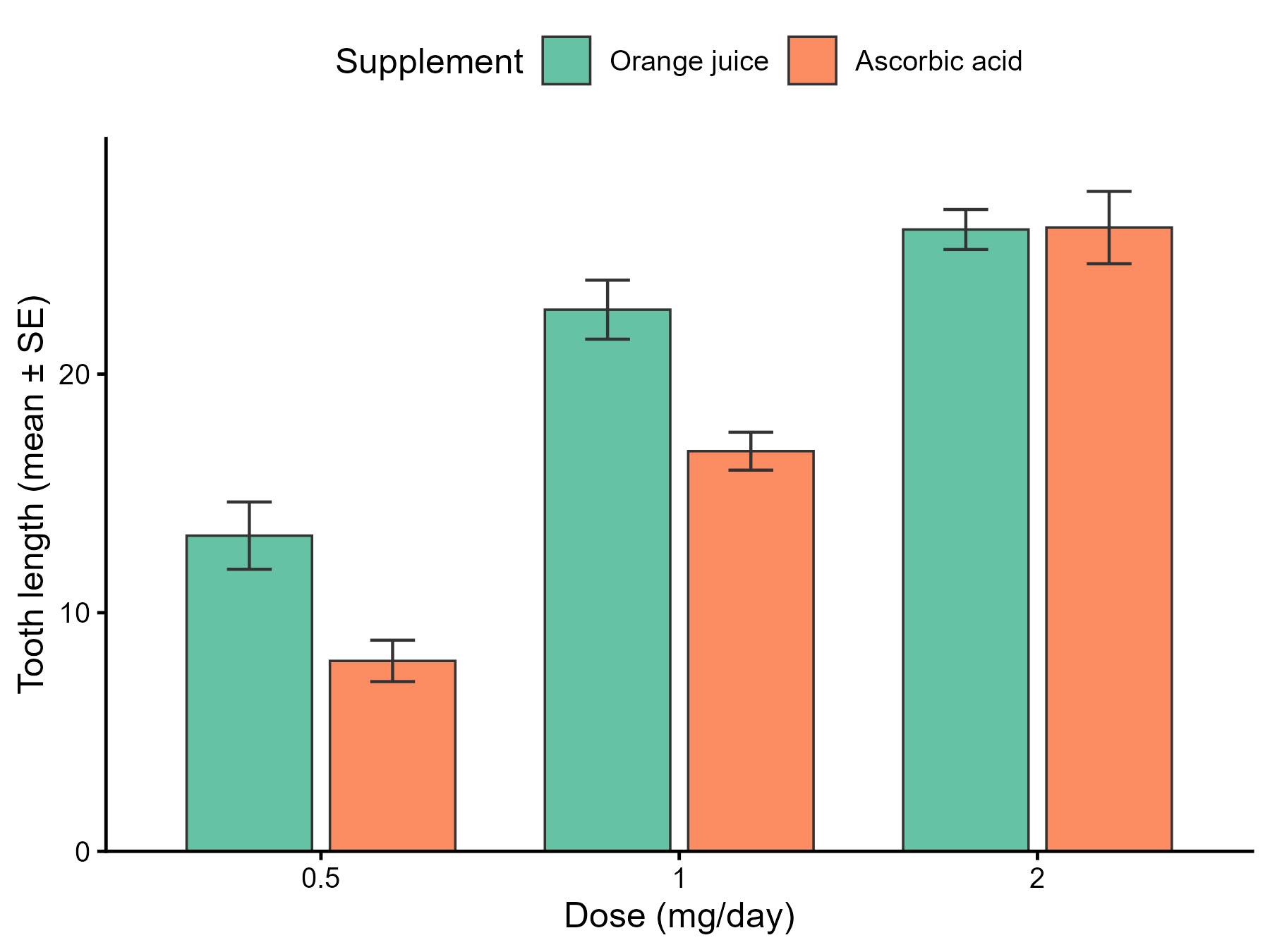
均值 ± 标准误柱状图(分组)
GAL-0005
用柱高表示各组均值,用误差线表示均值的标准误(SE),按两个分组因素并排排列。常见于论文,用来比较各组均值的大小及其估计精度。
图与代码
code/R/main.R
suppressPackageStartupMessages({
  library(ggplot2)
  library(dplyr)
})

d <- read.csv("data/toothgrowth.csv", encoding = "UTF-8")
d$dose <- factor(d$dose, levels = c(0.5, 1, 2))
d$supp <- factor(d$supp, levels = c("OJ", "VC"))

# 均值与标准误(SE = SD / sqrt(n))由代码从原始数据计算
s <- d %>%
  group_by(dose, supp) %>%
  summarise(mean = mean(len), se = sd(len) / sqrt(n()), .groups = "drop")

p <- ggplot(s, aes(x = dose, y = mean, fill = supp)) +
  geom_col(position = position_dodge(width = 0.8), width = 0.7, colour = "grey20", linewidth = 0.4) +
  geom_errorbar(aes(ymin = mean - se, ymax = mean + se), position = position_dodge(width = 0.8),
                width = 0.25, linewidth = 0.5, colour = "grey20") +
  scale_fill_manual(values = c(OJ = "#66C2A5", VC = "#FC8D62"),
                    labels = c("Orange juice", "Ascorbic acid")) +
  scale_y_continuous(expand = expansion(mult = c(0, 0.08))) +
  labs(x = "Dose (mg/day)", y = "Tooth length (mean ± SE)", fill = "Supplement") +
  theme_classic(base_size = 12) +
  theme(legend.position = "top")

ggsave("outputs/figure_r.png", p, width = 6, height = 4.5, dpi = 300, bg = "white")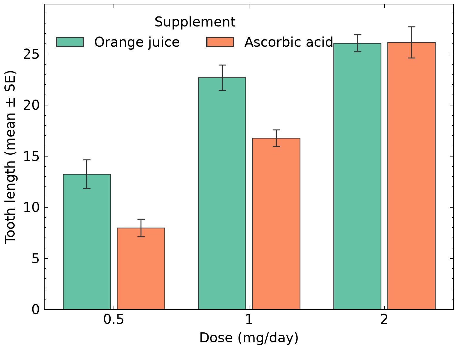
code/py/main.py
import numpy as np
import pandas as pd
import matplotlib.pyplot as plt
import scienceplots  # noqa: F401
from matplotlib.patches import Patch

plt.style.use(["science", "no-latex"])
plt.rcParams.update({"font.family": "sans-serif", "font.size": 11})  # 与 R 版(theme_classic 无衬线)统一

d = pd.read_csv("data/toothgrowth.csv")
doses = [0.5, 1.0, 2.0]
supps = ["OJ", "VC"]
labels = {"OJ": "Orange juice", "VC": "Ascorbic acid"}
colors = {"OJ": "#66C2A5", "VC": "#FC8D62"}
dodge, width = 0.8, 0.7

fig, ax = plt.subplots(figsize=(6, 4.5))
for i, dose in enumerate(doses):
    for j, s in enumerate(supps):
        y = d.loc[(d["dose"] == dose) & (d["supp"] == s), "len"].to_numpy()
        m = y.mean()
        se = y.std(ddof=1) / np.sqrt(len(y))  # SE = SD / sqrt(n),由代码从原始数据计算
        x0 = i + (j - 0.5) * dodge / 2
        ax.bar(x0, m, width=width / 2, color=colors[s], edgecolor="#333333", linewidth=0.6)
        ax.errorbar(x0, m, yerr=se, color="#333333", lw=0.8, capsize=3, capthick=0.8)

ax.set_xticks(range(3))
ax.set_xticklabels(["0.5", "1", "2"])
ax.set_xlabel("Dose (mg/day)")
ax.set_ylabel("Tooth length (mean ± SE)")
ax.margins(y=0.08)
ax.set_ylim(bottom=0)
ax.legend(handles=[Patch(facecolor=colors[s], edgecolor="#333333", label=labels[s]) for s in supps],
          title="Supplement", loc="upper left", ncol=2, frameon=False)
ax.tick_params(axis="x", which="minor", bottom=False, top=False)  # 分类横轴不要次刻度
fig.savefig("outputs/figure_py.png", dpi=300, facecolor="white")
什么时候用
- 比较多个组的均值,并同时表达均值估计的不确定性
- 论文或报告中对均值差异做简洁概括
- 两个分组因素(如剂量 × 处理方式)的并列比较
常见误用
- 柱状图只呈现均值与误差线,会掩盖数据的实际分布、离群点和样本量;样本量不大时建议叠加原始数据点或改用箱线图
- 标准误(SE)描述均值估计的精度,标准差(SD)描述个体数据的离散,二者不能混用;图注必须写明误差线是 SE 还是 SD
- 误差线不重叠不等于差异显著,重叠也不等于不显著;差异需用相应的统计检验判断
- 柱状图纵轴应从 0 开始,截断纵轴会夸大组间差异
数据与下载
数据:R 内置数据集 ToothGrowth(datasets 包)(R 内置数据集(随 R 分发,GPL-2 | GPL-3))。60 只豚鼠的成牙本质细胞长度(len,R 文档:负责牙齿生长的成牙本质细胞的长度),分为 3 个维生素 C 剂量(0.5、1、2 mg/天)和 2 种给药方式(橙汁 OJ、抗坏血酸 VC),每个组合 10 只。均值与标准误(SD/√n)由代码从原始数据计算。
下载包 sha256:0f7e2b5aa1612ed0ef6eedd626ae05eabc171ef8d21a260a47410665bf219dd7